ArcGIS Pro
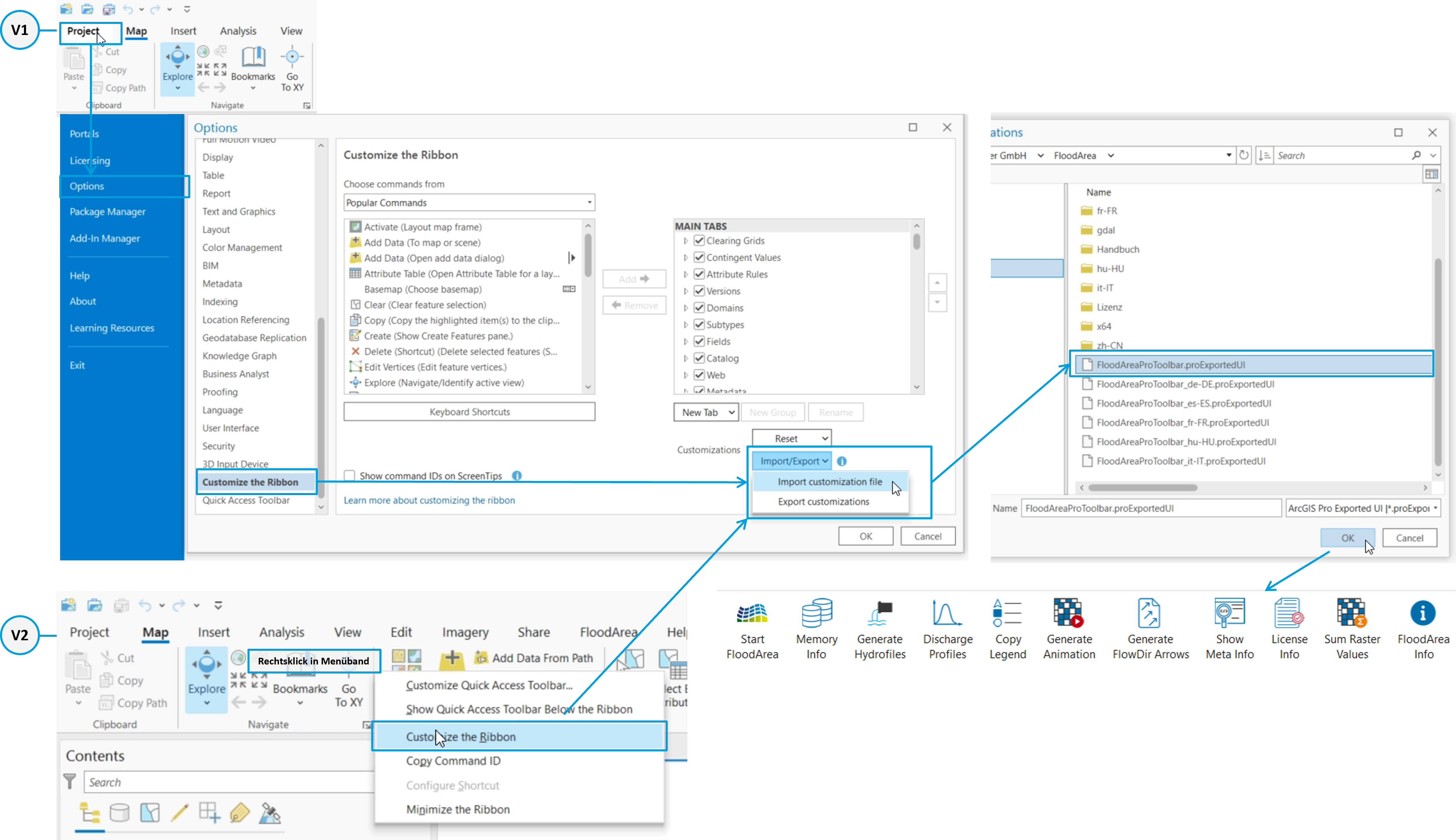
FloodArea HPC 11 can be used in ArcGIS Pro through both the ribbon menu and the toolbox. Both methods provide access to all FloodArea HPC 11 functionalities. The tools are always executed through ArcGIS Geoprocessing. The following chapters describe the various functionalities in detail.
FloodArea HPC Licence
The required license key file is delivered as an xml file and can be copied to any location.
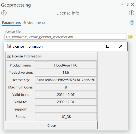
When the dongle has been activated (see Installation), you can specify and validate the license file under the menu item License Info.
After entering a valid license key file for FloodArea HPC 11, full functionality becomes available. Without specifying a valid license file in conjunction with the corresponding dongle, no calculation with FloodArea HPC 11 is possible.
Available Memory
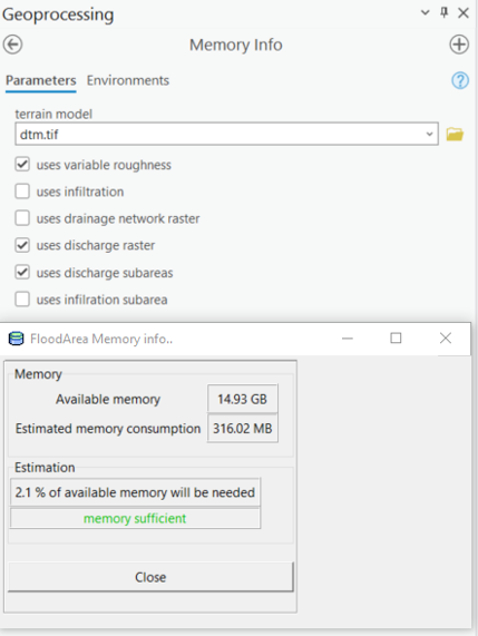
This menu item allows you to check whether the required memory is available. Please note that this can only be an estimate, as all other programs and the operating system permanently access the available memory. The memory specifications only include physical memory, as virtual memory should not be used if possible. Additionally, only the size of the terrain model as a rectangle, including NoData pixels, is considered (Extent). If the terrain model is not rectangular and thus has a proportion of NoData pixels, the required memory decreases accordingly.
You can specify either a raster layer from the current data frame or a raster dataset stored on the hard disk. If you select the option Load from disk, the selected raster will also be loaded into the data frame.
You also have the option to select different simulation options. Depending on the simulation configuration, memory requirements vary (combination of different options such as variable roughness, rainfall raster, rainfall subdomains, etc.)
Generate Hydrofiles
If you want to use the point input calculation function, this tool can help you create the hydrograph and coordinate files. To use it, you need a line feature class where the extraction point and injection point are connected by a line. In the Example data folder you’ll find a template that you can adapt to your project (Pay attention to the coordinate system):
When creating pump connections, the digitizing direction of the lines is crucial (starting point = extraction, end point = injection point). Here is an example of an attribute table:
The ID, which is written into the first column of the coordinate file is reassigned based on the order of the FID (first column in attribute table).
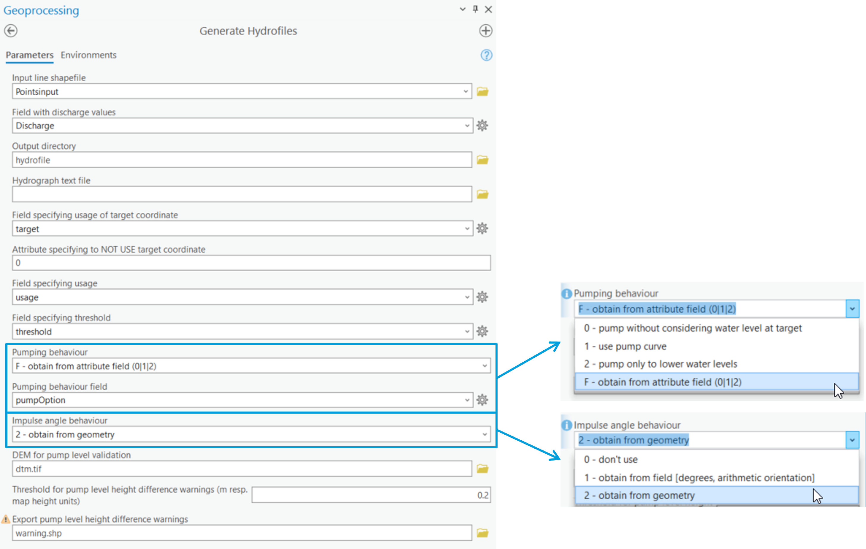
The tool can be used as follows:
Field descriptions:
Attribute column with flow information:
The water quantity to be pumped is in the Discharge column and is written to the Point input hydrograph (in m 3/s). If the value is positive, water is pumped out from the initial coordinate (negative value in hydrograph file). If you enter a negative value in the attribute column, injection occurs (positive value in the hydrograph file). Thus, a sign reversal takes place during generation.
Hydrograph text file:
A hydrograph text file can be specified as a template. The time steps (first column in each case) are then adopted. If no rainfall hydrograph is specified, the hydrograph has a time horizon of 8760 hours.
Attribute column with usage information for target coordinate:
Defines whether the extracted water quantity is fed in through the target coordinate (endpoint of the line) or completely removed from the simulation (starting point). This corresponds to the target column in the example feature class. Typically, the value for a pump connection is set to 1 and the value for a point input without target coordinate is set to 0 (default).
Attribute column specifying whether a pump connection should be used:
Distinction of which coordinates water should be pumped to (practical for different scenarios despite one shapefile, definition via 0/1).
Attribute column for threshold value:
Atribute column with minimum water level from which water should be pumped first (specification in cm). One application would be, for example, the inlet structure of a flood retention basin.
Setting the pump behavior:
The switch indicates which pump behavior should be used, i.e., whether the water levels between start and end coordinates should be compared (0, 2) or a pump characteristic curve should be used (1). Options 0, 1, 2 are applied to all line objects in the feature class. For option F, an attribute column in the feature class is used.
Setting the impulse angle:
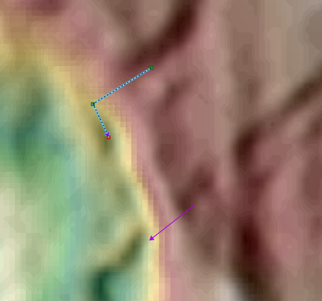
Here it is possible to read out the impulse angle from the geometry of the line. The direction vector of the last segment of a polyline is used. If a connection has only two support points, these are used for the impulse direction. However, you can add additional support points and thus modify the impulse direction. Examples of this are shown in the figure below.
Specifying a height model and threshold:
To ensure that the pump connections pump in the correct direction, the start and end pump points must be positioned correctly. This function allows you to check your pump connections for correctness. If the end point is higher than the start point, you will receive a warning message. The exported feature class allows you to quickly review the pump connections in question.
Start FloodArea HPC Simulation
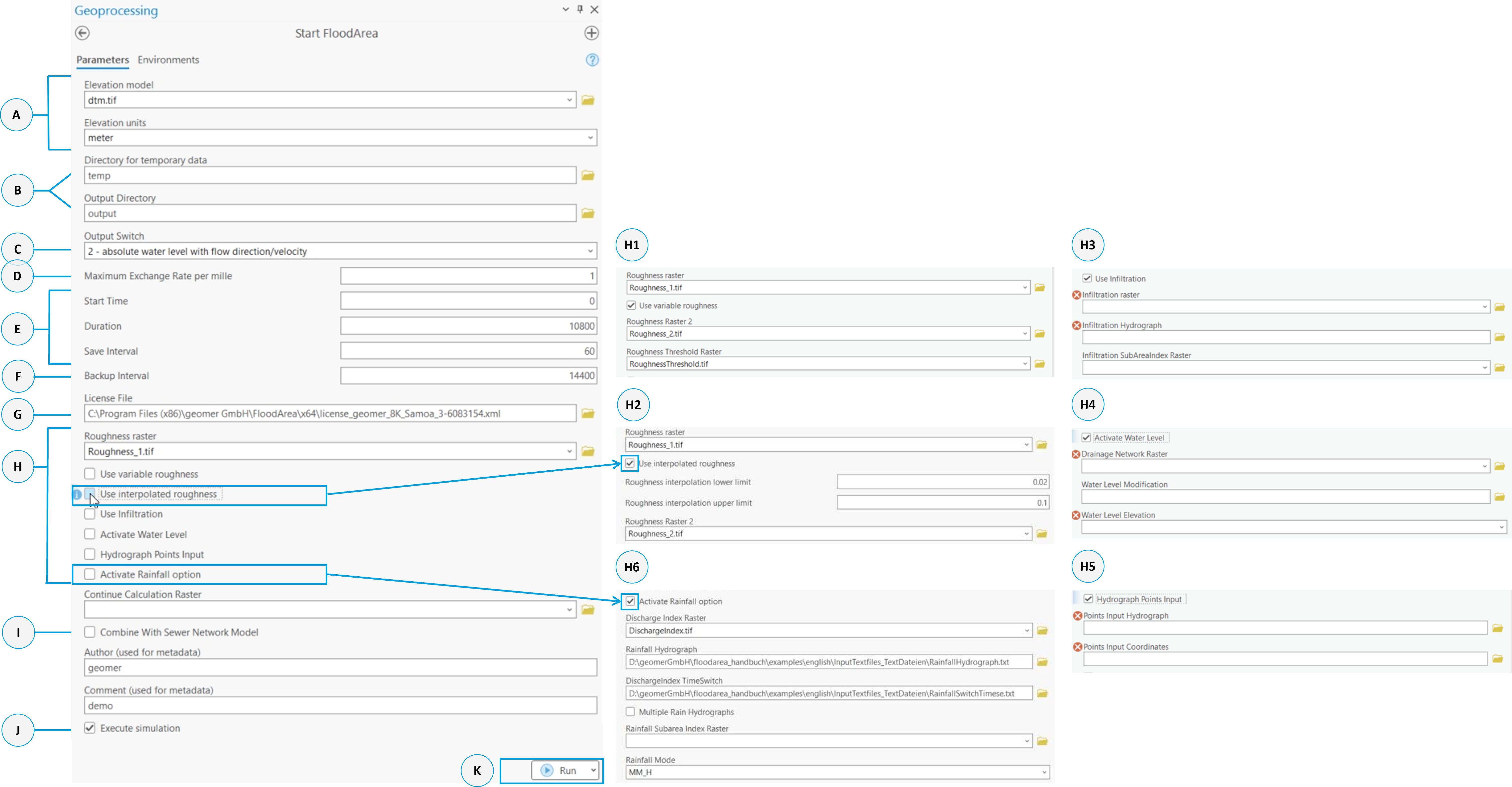
This menu item represents the core of FloodArea HPC 11. Under the menu item Start FloodArea Simulation, you’ll find the following geoprocessing field:
The data formats and specifications of the different calculation options are explained in the chapters Eingangsdaten and Calculation Options.
All fields marked with a red asterisk are mandatory. The different calculation options can be selected via checkboxes and freely combined. One of the three calculation options - Water Level, Point Input, or Rainfall - must be active.
Only the optional function Continue Calculation with Existing Grid does not need to be specifically activated.
The following parameter explanations also reference the structure of the fng.xml (see Starting FloodArea via XML ).
Field A: Basic Datandaten
Path to Digital Terrain Model, specifying height unit and cell size (required for every simulation).
XML: Paths - DTM_ras, General Settings - ElevationUnits und RasterUnits.
Field B: Output Options
The paths for temporary data and simulation results. The fng.xml is saved in the temporary data folder (see Starting FloodArea via XML). In the output directory, the simulation result rasters are stored in newly created folders named “output” (flood depth), “velocity” (flow velocity) and “direction” (flow direction). The output rasters are prefixed with “o”, “v”, or “d” at the beginning of the filename. The FloodArea HPC 11 log file and volume.txt are also written to this path. If the calculation option Point Input is activated, the file PumpVolume.pum is also stored here - see Reading Pump Volume.
XML: Output_dir und Temp_dir
Field C: Output Type
1 = Flood depth in water level (absolute height)
2 = Flood depth in water level (absolute height) + flow velocity and direction
3 = Flood depth in flooding depths (relative height)
4 = Flood depth in flooding depths (relative height) + flow velocity and direction
XML: GeneralSettings - OutputSwitch
Field D: Maximum Exchange Rate
This performance variable determines the duration of an iteration step together with the cell size (time step length = cell size * exchange rate/100). The duration of the iteration step indirectly determines what maximum calculated exchange amount can still be represented by the algorithm.
In other words, the exchange rate influences what proportion of the current cell content can be passed on to neighboring cells during one iteration step. If the cell size of the input rasters is changed, the algorithm adjusts its time step to maintain stable maximum representable propagation speed.
The lower the duration of the iteration step is:
The less water volume can be exchanged between two cells according to flow conditions
The more iteration steps are needed to transfer the same volume of water
The more iteration steps are needed within an iteration interval
The longer the duration of an iteration interval and thus potentially the simulation time
However, the more accurate the simulation results
If the values specified here are relatively large, depending on environmental conditions, “wave sloshing” can occur in the model. While these instabilities don’t lead to a termination of the simulation run, in extreme cases they can distort the results due to excessively high water levels in individual cells. Experience shows that values between 1 and 5 provide the best results. The smallest possible input value is 1. Larger exchange amounts (maximum possible is 100) only make sense if you want to significantly reduce the simulation time for preview purposes. For this purpose, it is also advisable to calculate with a coarser grid resolution.
XML: GeneralSettings - MaxExchangeQuantityPromille
Field E: Simulation Time and Storage Interval
Time is specified in seconds. Simulation start time is normally set to 0, unless continuing a previous calculation (Continue Calculation). The Save Interval corresponds to the interval at which simulation results are saved
XML: TimeSetup (in seconds)
Field F: Backup-Interval
FloodArea HPC 11 creates backup files during simulation (written to the output directory). During each FloodArea HPC 11 calculation, backup files are written at regular intervals to save the current calculation status. If a calculation was not completed successfully, e.g., due to early termination by the user, the simulation can be restarted from the last backup. If a backup file from a previous calculation exists in the specified temp folder, it is automatically read and used to start the new calculation.
Note
If a simulation was terminated at 80% of the calculation and the last backup was saved at 75%, a new calculation based on the backup file will continue from 75%.
This only happens if the same output directory is specified for the new calculation. The default value for the backup interval is 14400 (equivalent to 4 real time hours) and is interpreted as seconds of real calculation time. The specification of 14400 seconds thus corresponds to every 4 hours. Only the current backup file is retained. Depending on the simulation being performed, it may be useful to adjust the backup interval.
Field G: License File
Here the path to the license file is specified
XML: Paths - LicenseFile_xml
Field H und I: Calculation Options
Calculation Options As soon as you activate an option by checking it, a menu field opens for the additional required inputs. The data formats and specifications of the calculation options are explained in their respective chapters Water Level - Point Input - Rainfall - Optional Inputs.
Fields J und K: Executing the Simulation
If the Execute simulation checkbox is checked, FloodArea HPC 11 will start immediately when clicking RUN (Field K). If the checkbox is not checked, only the fng.xml is written to the folder for temporary files (Field B). With this file, FloodArea HPC 11 can then be started from the command line (see Starting FloodArea via XML).
Continue Calculation
If the simulation is terminated prematurely during execution, there are three ways to continue the calculations:
Backup: If a backup folder exists in the results directory, you can restart the simulation from the history in GIS or the command line (fng.xml in output folder). FloodArea HPC 11 automatically accesses the backup. The continuation time step depends on the backup’s save interval.
Under the optional function Continue Calculation with Existing Grid in the Start FloodArea tool, you can select a flood depth raster from the output folder (e.g., o060.tif). You must also adjust the start time according to the save interval. With an interval of 60 seconds and o060.tif, the start time would be 3600.
Note: If you use changing discharge coefficient rasters with the Rainfall calculation option: Beregnung you must select the raster that matches your time step.
Using the Show Meta Info / Continue Calculation function, you can read in a flood depth raster. The necessary settings are taken from the metadata. Of course, paths from meta date must not been changed meanwhile. There is no possibility to manually change the discharge coefficient raster. A change only occurs when the time step in RainfallSwitchTimes.txt specifies it.
Discharge Profiles
The function Discharge Profiles performs discharge hydrograph calculations using the simulation results. These calculations can be used, for example, to determine the requirements for possible flood retention measures (volume, maximum discharge rate).
Discharge Profiles Input
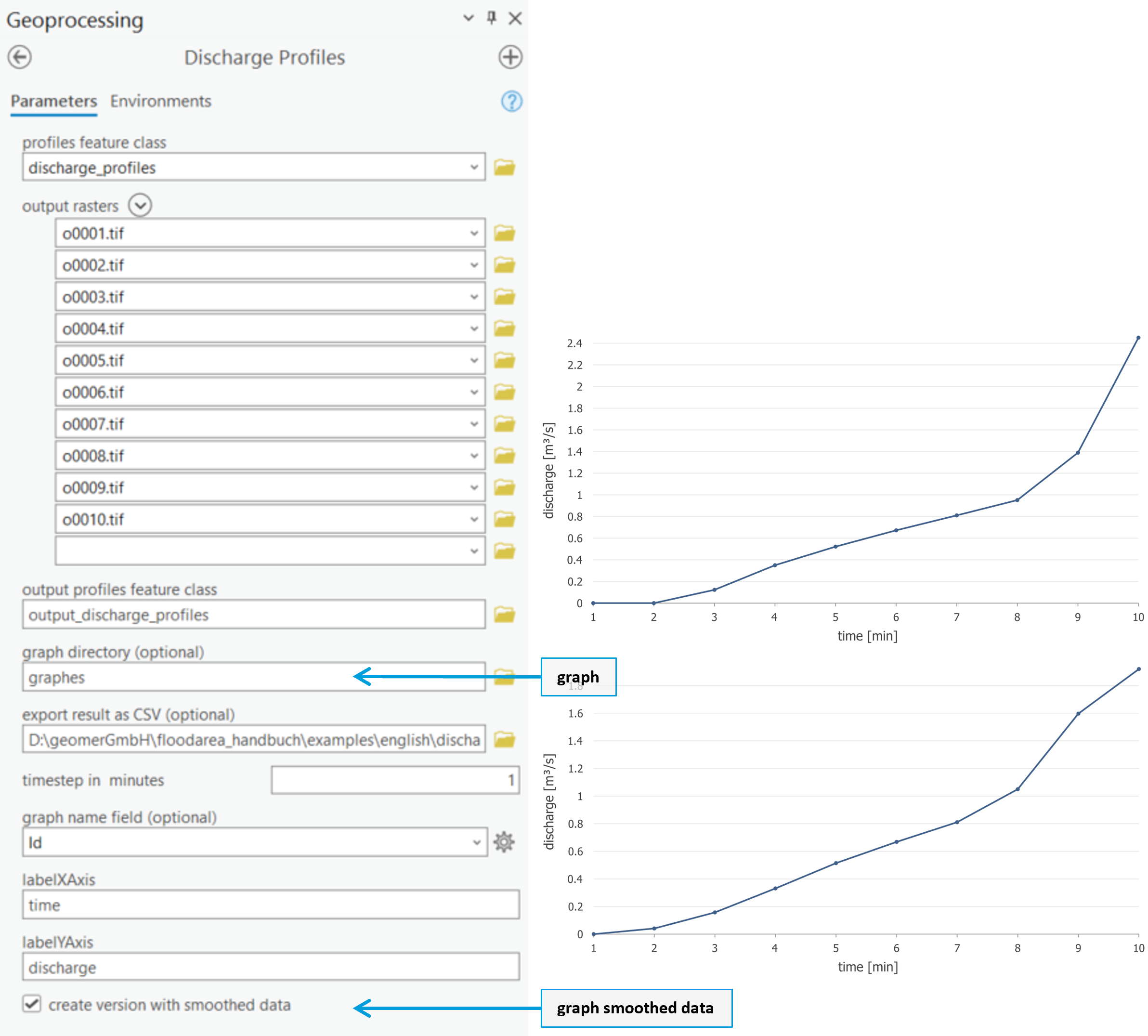
A polyline Feature-Class is required as data input. The discharge is determined along these lines. When digitizing the discharge lines, care should be taken to ensure that there is a clear flow direction without strong turbulence or backwater at this location.
Output Raster
The calculation of discharge requires the simulated flood depths in the correct temporal sequence. Since the tool also needs and automatically accesses the associated flow velocities and flow directions, the folders output, velocity and direction must be present in the same structure as generated by FloodArea HPC 11.
Output Discharge Profiles
A new shape is generated with the discharge lines. The tool writes the total discharge volume (unit of the dtm raster in cubic), the maximum discharge peak, and the individual discharge rates (unit of the dtm raster in cubic per second) for each time step into a new column in the attribute table of this shape. Please consider the time step length that you set during the simulation if you want to perform calculations with the individual values.
Output Diagrams
If desired, a graph could be output for each discharge line for the entire simulation time by specifying a file path.
Export Result as CSV
This is an optional input and exports the attribute table of the output discharge profiles to a .csv file.
Time Step of Output Raster in Minutes
To correctly calculate the total volumes from the individual time steps, the time step must be specified here in minutes.
Attribute Column for Diagram Labels
Optionally, you can select an attribute column from your discharge profile Feature Class with profile names or designations. These are used for the profile headings in the graph itself and in the filename.
Axis Labels for X-Axis and Y-Axis
Here you have the option to customize the axis labels. The default settings are time (x) and discharge (y).
Generate Version with Smoothed Data
With very small time steps, for profiles in areas with ambiguous flow direction such as backwater areas or directly behind pump connections, the discharges may show strong fluctuations. This function applies a weighted average with middle emphasis over 3 minutes, which smooths the peaks.
Generate Animation
Using the functions under the menu item Create Animation, you can visualize the temporal progression of a flood in the form of a video. A series of JPEG images and an animation file in MP4 format can be created. First, load the flood depths you want to create an animation with and desired background maps into a new ArcGIS Pro project. Using the Copy Legend tool, you can adjust the legends of the flood depths. Arrange the rasters in the desired order. The first raster (e.g., o0001.tif) should be on top. Then select all rasters and group them into a folder. To do this, select all rasters and create a new folder by right-clicking on Group. Next, create a layout for the animation. You can add legends, north arrows, or other map elements to your layout as desired, pan to the desired map section, and adjust the scale. When the layout is ready, open the animation tool.
Enter the desired layout in Input Field A. The previously grouped raster layers to be animated are specified in Input Field B. The storage location for the animation is defined in Input Field C. There are different ways to display and place the simulation time in the animation. Using the drop-down menu at Input Field D, you can choose between 6 different options:
0 = do not add
1 = display at current position
LR = add bottom right
LL = add bottom left
UL = add top left
UR = add top right
The storage location for the individual images is given in the messages at the end of the tool, or you can find the images in this directory on your PC: %TEMP%
In Input Field E, you can modify the text template Simulation time: {} as desired. However, it’s important that the curly brackets {} remain intact.
The resolution settings can be specified in Input Field F. Depending on how long you want the video to be, you can specify the frames per second (Input Field G). If you don’t want to delete the intermediate images (individual frames per time step), you must check the box (Input Field H). Otherwise, only the video will be saved. The storage location of the images is shown in the messages at the end of the tool.
Copy Legend
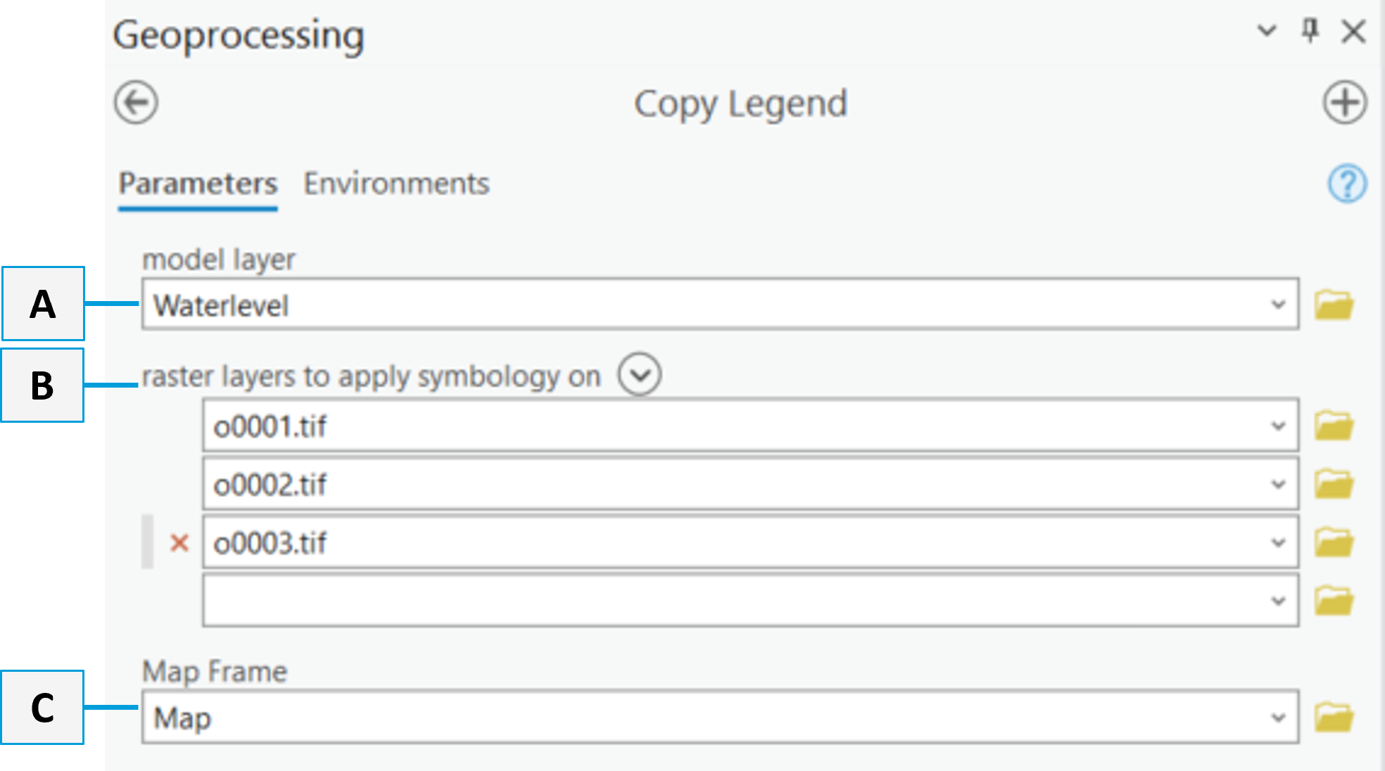
This menu item provides a tool to assign an identical legend to different raster layers. This is especially necessary when you want to compare results from different calculation runs or for creating animations.
First, select the layer with the desired symbolization in Input Field A. Then enter all your rasters to be modified in Input Fields B. Finally, the map must be specified in Input Field C and then the tool can be started.
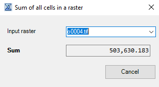
Sum Raster Values
With this function, all values for any raster layer are summed up. For example, if flood depths are present and horizontal and vertical units are identical, the total existing water volume is output. This allows volume balancing for the respective time step of the raster.
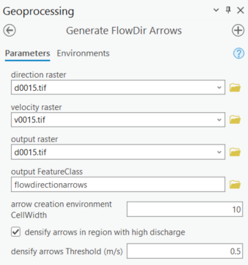
Generate Flow Direction Arrors
Using this tool Generate Flow Direction Shape, flow directions are created as points that can then be displayed as flow arrows with corresponding direction. You must specify the respective flow direction, flow velocity, and flood depth raster. The output directory is saved as a Esri Feature Class in a geodatabase (.gdb). In the setting cell size for arrow generation, you can specify a cell size to thin out the flow arrow density. If you want the flow arrows to become denser at high flow velocities, you must check the following box. In the last setting, a threshold value can be specified. When the velocity of the raster cell exceeds the threshold value, half the value of the surrounding cells is used.
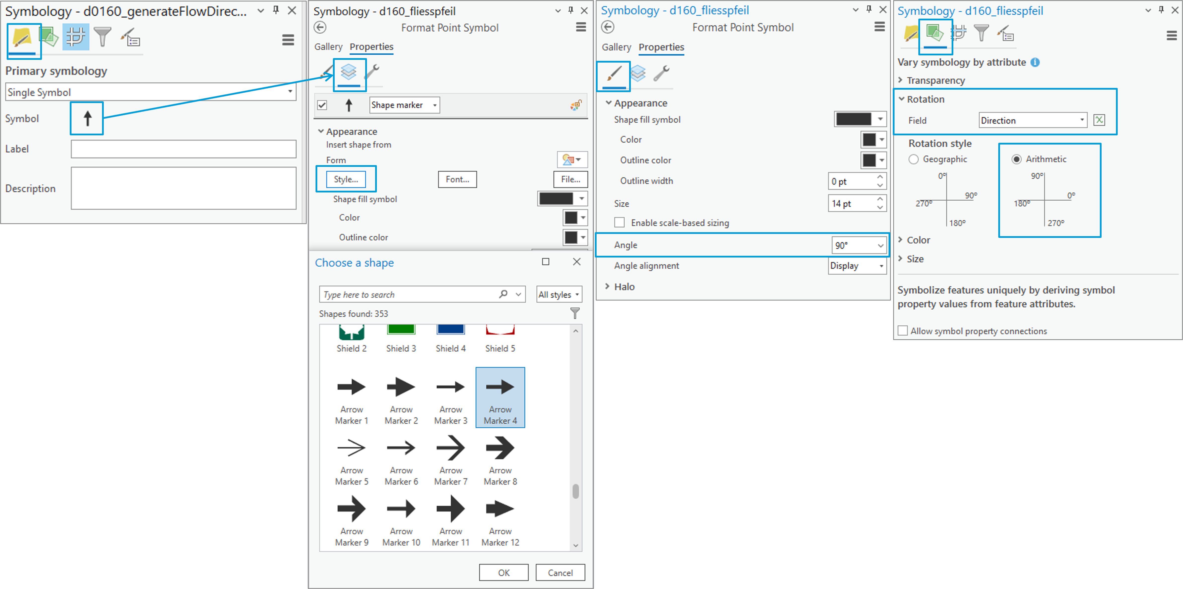
When you want to display the point Feature Class as arrows, you can adjust the symbolization as shown in the following figure:
Open the Symbology tab in ArcGIS Pro.
Select an arrow as a Single Symbol and click on the symbol.
Under the settings in the layer tab, you can adjust the style again.
Switch to the Symbol tab in the settings and change the Angle to 90°.
In the Vary Symbolization by Attribute tab, expand the Rotation point. Select Direction in the field and choose Arithmetic for the Rotation Style.
Show Meta Info / Continue Calculation
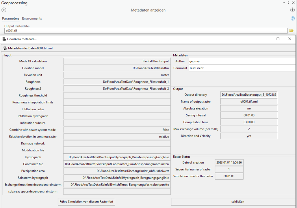
Under this menu item, you can view the creation information (FloodArea HPC 11 metadata) and continue calculations that were previously started.
This can be based on either a flood depth raster layer loaded in the current map frame or a flood depth raster stored on the hard drive.
In the input display area, the simulation parameters used to generate the respective raster are listed. Under the output area, you’ll find the simulation parameters that were specified during the simulation. If a switch (checkbox) was activated in the main menu or under Additional Settings during the simulation, the value “Yes” is entered here. If not, the value “No” appears. Not all switches are listed here, but their status can be derived from those given.
The Close button ends the display of metadata in the system. If you want to continue the simulation, you can do so using the switch “Continue Simulation from this raster,” which will directly resume the simulation. However, this only works provided that the paths have not changed in the meantime. Note: If a backup file exists in the results folder, this will be used for continuing the simulation.
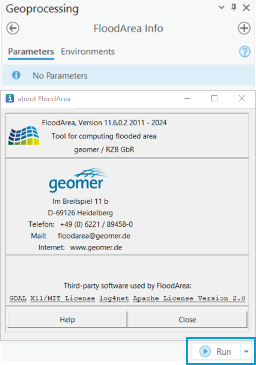
FloodArea Info
Here the version number and service addresses are displayed. You simply need to execute this tool and the info field will appear.
