ArcMap

The hydraulic modeling with FloodArea ^HPC 11 in ArcMap can be done via the GUI and via the toolbox. The GUI and toolbox have different functionalities, which are described in the following sections.

GUI

Activation

After installation and activation of the extension, a new toolbar is permanently available in ArcMap. Before you can use it, you must activate it by clicking the box in the Customize menu (Extensions and Toolbars).

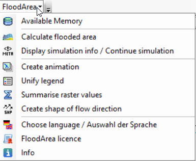
After loading the toolbar, this toolbar is available like all others. The available sub-items are shown in the following figure.

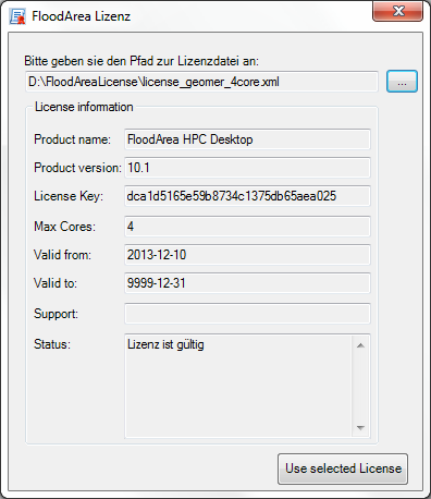
FloodArea License

Here the license for the FloodArea extension is either displayed, specified or changed.

As long as “DEMO” is displayed as license number, FloodArea works in demo mode, so all results are watermarked. In oder to leave the demo mode, you need a valid license file and a USB dongle.

The required license key is delivered as xml-file and can be copied to any place. If the dongle is activated (see Installation and License), the license file must be specified in the FloodArea toolbar to use the full functionality of FloodArea in ArcMap. You can access the corresponding dialog by selecting the item FloodArea License from the FloodArea menu.

After entering a valid license key file for FloodArea, the full functionality is available.

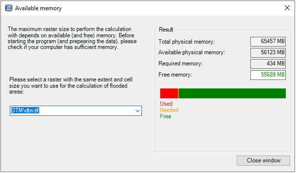
Available Working Memory

This menu item can be used to check whether the required working memory is also available. Please note that this can only be an estimation, since all other programs and the operating system also permanently access the available memory. The memory specifications only include the physical memory, since the virtual memory is not recommended to be used if possible. You have the option of specifying a raster layer from the current data frame or a raster data set available on the hard disk. If you select the option Load from disk, the selected raster is then also loaded into the data frame.

Calculation of Flooded Areas

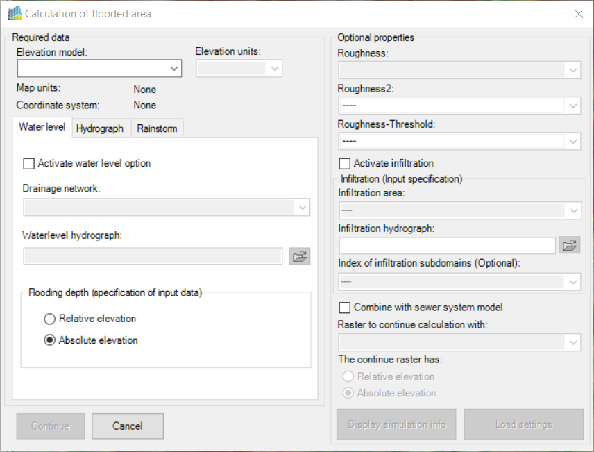
This menu item represents the core of FloodArea ^HPC 11. The menu item Calculate FloodAreas leads to the following dialog box:

The preconditions of the simulation are explained in the chapter Input data. The input of a terrain model and the selection of the height unit is mandatory. All other calculation options can be freely selected.

The calculation option to be used must be selected by checking the Activate…option. The activated options are marked with a ‘*’. One of the three calculation options Water level, Hydrograph or Rainstorm must be active. All three calculation options can be combined as desired. Only the optional functions Roughness or Calculation Grid do not need to be activated separately.

The data formats and specifications of the calculation options are explained in the respective chapter (Water level - Point injection - Irrigation - Optional functions).

The data can either be taken from the list of loaded raster layers or from disk.

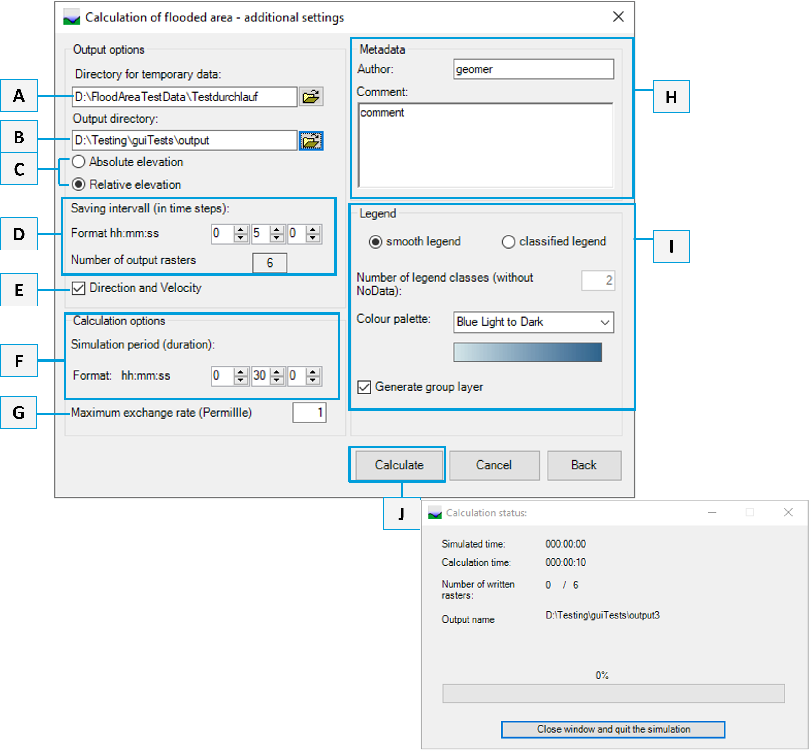
Additional Settings

Before the user can continue, the program checks the entries for plausibility. If there are any discrepancies, the user is notified of any problems or is asked to provide additional information. The check is carried out, for example, with regard to missing or incorrect entries. The button is only activated again when the plausibility is established.

Field A and B:

Working directories for temporary data that are generated at the beginning of the simulation and the output data. In the output folder another folder named “output” is automatically created, in which the result grids are stored. The result grids of the flood calculation itself are named after the pattern o + four-digit number (o0001.tif, o0002.tif etc.). If the selected grids do not already exist, they are created automatically.

Field C:

The output units of the calculation results can be in water level (absolute heights, usually this is the height above sea level) or in relative heights (flood depths). The units correspond to those of the terrain model entered.

Field D:

Furthermore the storage interval can be specified. The smallest time unit is one second.

Field E:

Checking the box for flow direction and flow velocity, grid data necessary for the creation of flow direction shapes are generated. Please note that this option generates three grids instead of one per calculation step. Especially when using this option, you should make sure that there is enough disk space available (in other cases, of course, as well). The additionally created rasters are stored in the output folder in separate folders named “velocity” and “direction”. The file names will start with “v” or a “d”.

Field F:

Under the item Calculation options the total calculation duration can be entered. If a simulation is to be continued, the duration is extended by the value entered here.

Field G:

The Maximum exchange rate specifies the maximum amount of the current cell content that can be passed on to the neighboring cells during one iteration step (in promille). The value specified here indirectly influences the simulation speed, since the model reduces the duration of the iteration interval in order to fulfill this condition. If the values specified here are relatively large, a “ripple” can occur in the model depending on the environmental conditions. These instabilities do not lead to a termination of the simulation run, but in extreme cases they can lead to an interruption of the simulation run, since too high water levels in individual cells falsify the results. Experience shows that values between 1 and 5 give the best results. The smallest possible input value is 1 (corresponds to 0.1%). Larger exchange quantities (a maximum of 100 (10%) is possible) are only useful, if you want to shorten the simulation time significantly in the sense of a preview. For this purpose, it is advisable to calculate with a coarser grid.

Field H:

FloodArea uses the Metadata concept of ArcGIS to store information about the rasters created during the simulation. Some of this information is generated automatically (like the simulation duration), others can be entered here like an author or scenario information etc.

Field I and J:

Here you can define the Legends for the output grid layers according to the ArcMap options. The value for NODATA is set to transparent by default. You can choose between a smooth legend or a classified legend and define a number of legend classes. The color ramp selection list also provides the option to load own color ramps. All generated raster layers receive the same display symbols. Finally, the Generate group layer option can be activated to add the calculated result grids as a group to the list of loaded raster layers. The group gets the name of the output grid followed by “Group”.

Use Calculate (J) to save the settings and start the calculation. Pressing the Cancel button discards the new entries.

Calculation Process

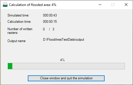
During the simulation, a window opens that shows the progress of the simulation. As this window is opened in the foreground during simulation, the ArcMap window cannot be used.

If ArcMap is closed during the simulation, the FloodArea simulation will also be quit. In this case, the simulation can be restarted using the FloodDepth Grid that was written out last - see option Continue Calculation.

The simulation settings are written to the specified temp folder in the file fng.xml.

A backup is written to the specified output folder during simulation. The frequency of the backup intervalls can not be set in the GUI. The backup is written every four hours (processing time). A log file is also written to the output folder.

Display Creation Info

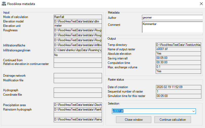
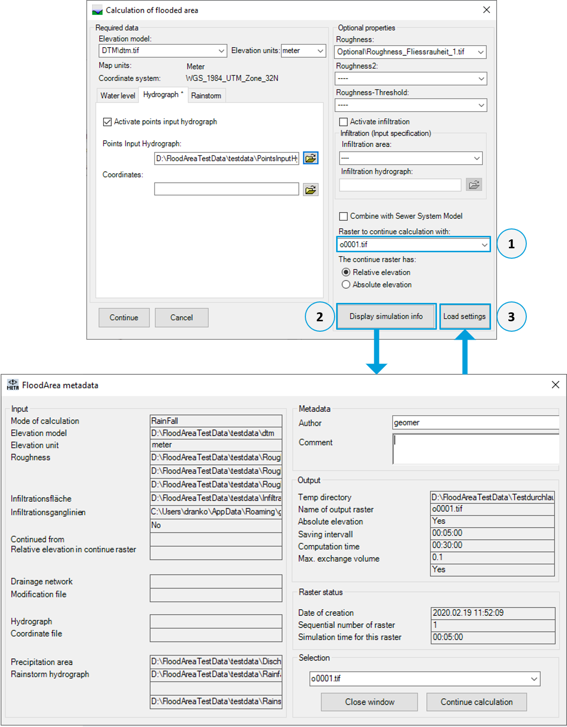
Under this item, the creation information (FloodArea metadata) can be displayed and calculations that have been started can be continued.

For the continuation of an aborted simulation you can either load a flood depth grid layer from the current map frame or a flood depth grid stored on your hard disk.

The simulation parameters used to generate the respective grid are listed in the input section. The output section shows the simulation parameters which were specified during the simulation. If during the simulation in the main menu or under More settings a checkbox was activated, the value Yes is entered here. If this is not the case, the value No appears. Not all switches are listed here, but their status can be derived from the ones given.

Close window terminates the display of metadata and returns to ArcMap. With the button “continue calculation” you can switch to the main dialog (see below). The grid used for further calculation is automatically entered into the dialog.

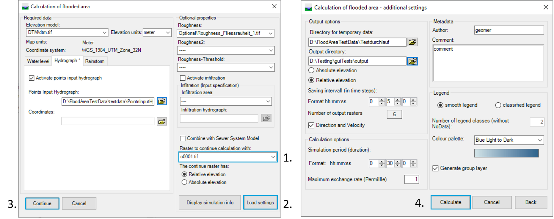
The button Load settings in the main menu reads the settings from the metadata of the selected grid and writes them into the flood simulation dialog. Otherwise, the settings of the last calculation or already specified data are used. On the other hand, the settings of the More Settings dialog are always automatically applied when a further calculation grid is specified, so that, for example, the same legend and the same saving interval are selected. If a change of the respective settings is desired, these must be made accordingly.

Create Animation

With the help of the functions under the menu item Animation, the temporal course of a flood can be visualized better than it is normally possible with ArcMap. A series of JPEG images and an animation file in MP4-format can be generated.

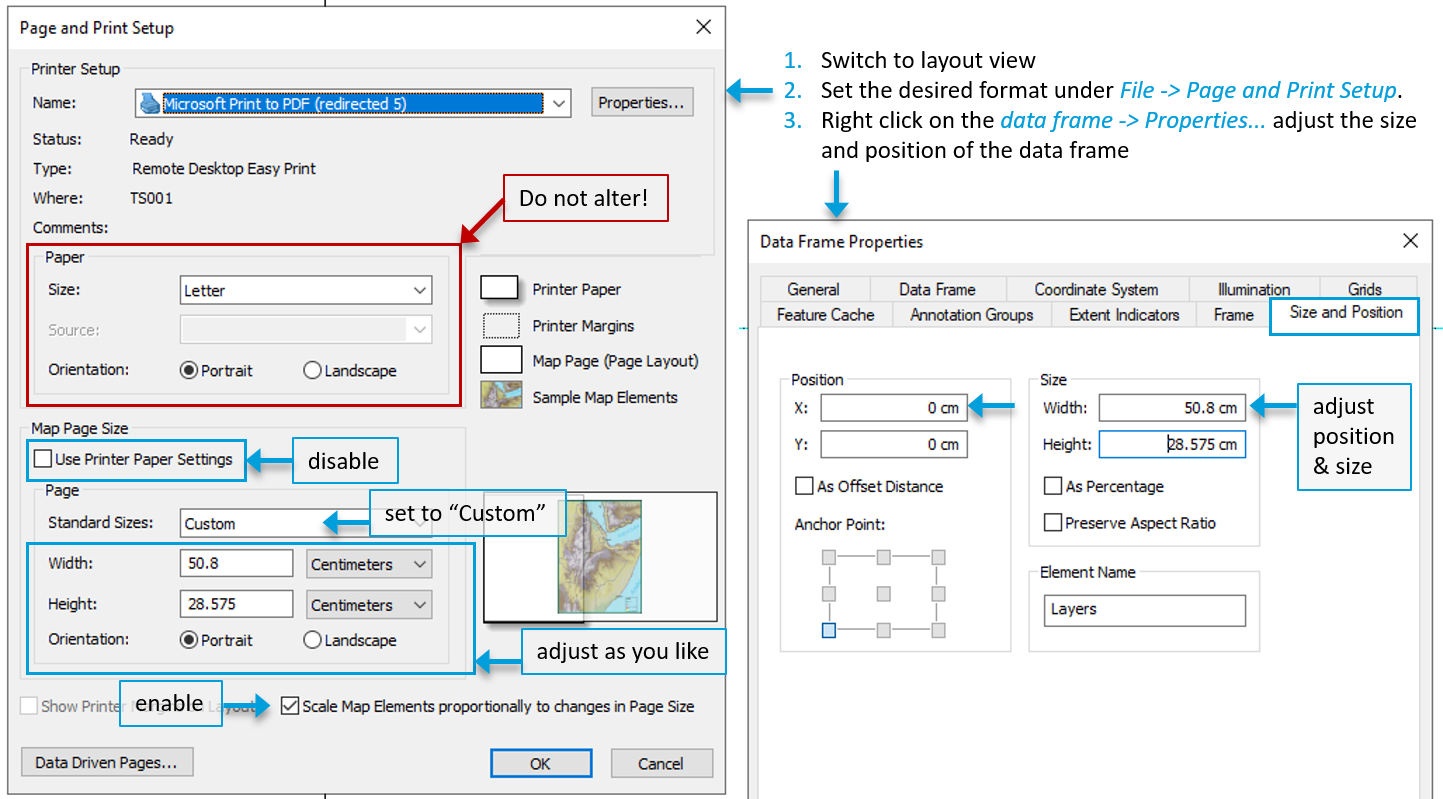
First of all, the inundation depths with which an animation is to be created and desired background maps are loaded into a new ArcMap document. Via the tool Assign same legend you can adjust the legends of the flooding depths. The next step is to switch to the layout view and set your format as desired under File - Page and Print Setup… . The procedure is shown in the following illustration.

You can insert legends, north arrows or other map elements into your layout as you wish, pan to the desired map section and adjust the scale. When the layout is ready, open the animation tool.

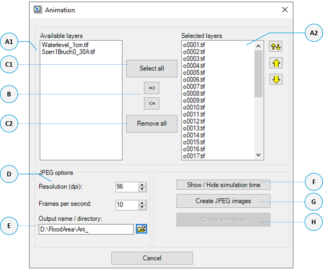
The layers to be included in the animation are managed in lists A1 and A2. From the list of available layers (A1), individual layers (via the switch B) or all layers at once (via the switch C1) can be selected. Accordingly, the layers can also be removed from the list of selected layers individually (switch B) or as a whole (switch C2). In both lists, a selection of several layers is possible. By holding down the Ctrl or Shift key, you can select one or more layers. In the list on the right hand side, you can modify the sequence of the screens to be generated by arranging the layers in the appropriate order. The buttons and move selected layers up and down in the list. Pressing the button reverses the entire sequence of the layers. You can select and reorder all layer at once as well.

The list of FloodArea layers appears in reversed order compared to the arrangement in the legend of ArcMap. This is because the last layers drawn in ArcMap must also be exported last when the animation is created. Reverse the order via the button ! The list is processed from top to bottom, while the table of contents of ArcMap is drawn from bottom to top.

Note

You can deactivate and group the flooding depths in the table of contents. It is only important that the group is activated. The background maps or hillshades should be activated.

In the input fields D the quality of the generated JPEG images and animation is defined. A lower JPEG quality reduces the size of the generated images and animations. The Frames per second input fields define the playback speed of the generated MP4-file. In the input field E the directory in which the generated images/movies are stored and the names of the files to be generated are defined. With input field F the simulation time of each FloodArea raster layer in the image/movie, read from the metadata, can be optionally displayed or hidden.

As soon as an output name has been entered, the simulation time can be displayed (input field F). This is read from the metadata of the inundation depths and appears at the bottom left of the layout when the field is activated. The format and location of the simulation time can be adjusted manually! To do this, you have to close the animation tool (via the Cancel button) after you have activated the simulation time. Now you can click on the simulation time and move it. In order to adjust the font, size and colour, do right click -> Properties… -> Change symbol (as with other text elements). Then open the animation tool again and continue (you have to set the fields D and E again).

Next, use the Switch G to create the JPEG images. The same number of images will be created as the number of result grids in the list of selected layers. The creation of an animation file can only be started after the JPEG images have been generated by the switch H. It is important that after the JPEGs have been created, the animation tool is NOT closed again, but the animation file is created directly! Otherwise the tool will not find the JPEGs again and they have to be created again.

If the animation file has been created successfully (it is located in the specified directory), the animation tool can be closed.

Unify Legend

This menu item provides a tool to assign an identical legend to different raster layers. This is especially necessary, if you want to compare results from different calculation runs.

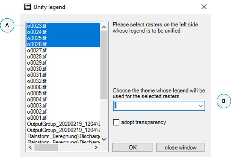
First select all layers in the List A which should get the same legend. Then select a layer that already has the desired legend display in the selection list B. Choose OK to accept the selection and all selected layers are displayed with the same legend.

Sum of All Cells in a Raster

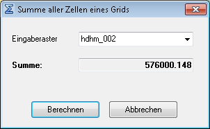
This function adds up all cell values of a raster layer. If, for example, flood depths exist and horizontal and vertical units are identical, the existing total water volume is output. This allows the analysis volume balances.

Create Flow Direction Shape

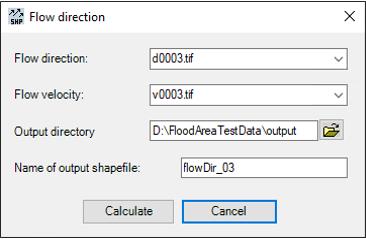
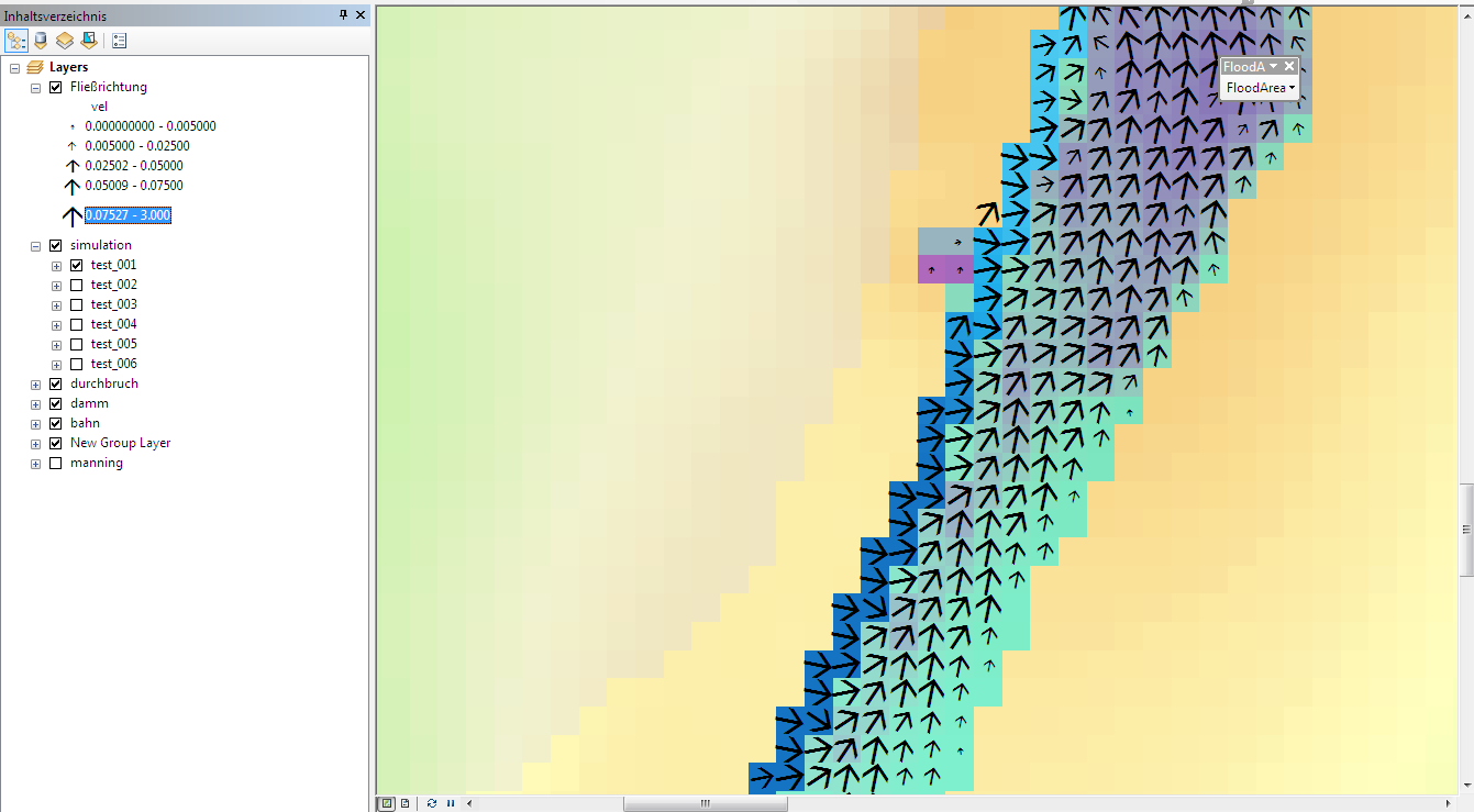
A shape file can be generated with flow direction information. Herefore the grids are used, that were calculated when the option Direction and Velocity was activated in the Additional settings dialog. To do this, the corresponding grids must be selected and a name for the output must be specified. The files are located in the same directory as the output files with the water levels. Please note that the required input files will only be created if this has been set under Addtional settings.

If the direction arrows are displayed too large or small, this may be due to a missing or the incorrect entry of map units and the reference scale in the map frame properties.

In other cases you should use the advanced options of the legend to adjust the reference scale. The default scale is 1:1000. This scaling is optimized for the provided demo area.

According to the internal management of the neighbouring grid cells, it is possible to display 16 different directions. This results in a relatively uniform flow pattern. However, it should be noted that the flow direction specifications are snapshots of the entire sumulation time. It is therefore wise to display several situations, especially in situations with strongly changing flow conditions.

Language

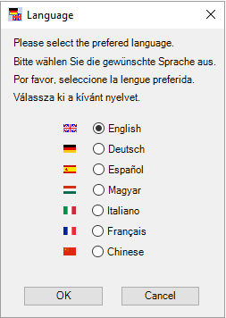
FloodArea contains the option to change the language of the dialog boxes, help texts and messages between German, English, Hungarian and Spanish. After pressing the OK button, the working environment of FloodArea is immediately changed to the selected language. This does not apply to the language of the ArcMap interface.

Info

The version number and service addresses are displayed here. This dialogue also includes the Help button, by clicking this button will open user manual.

Toolbox

Mit der FloodArea-Toolbox ist es möglich, die Funktionalitäten der FloodArea-Extension über die Arc-Toolbox zu nutzen. Um die FloodArea-Toolbox verwenden zu können, muss die Lizenzdatei als entsprechender Parameter angegeben sein.

Activation

The initialization takes place automatically with the installation of FloodArea. Before the toolbox is available in ArcMap or ArcCatalog, it must be loaded from the installation folder of FloodArea using the methods common in ArcGIS.

Start FloodArea ^HPC 11 Simulation via Toolbox

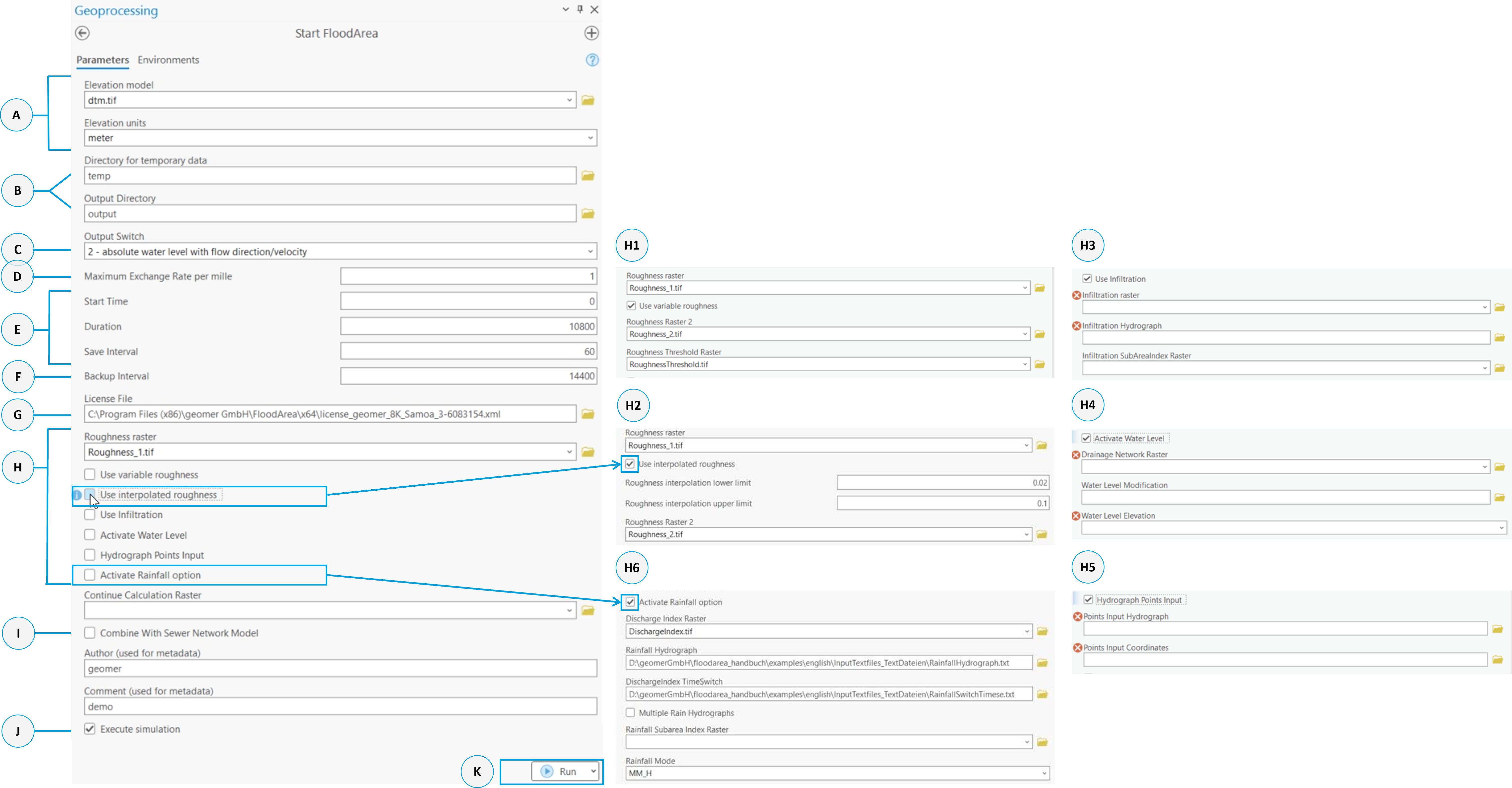
This menu item represents the core of FloodArea ^HPC 11. Under the menu item Start FloodArea Simulation, you will find the following geoprocessing field:

The data formats and specifications of the different calculation options are explained in the chapters Input Data and Calculation Options.

All fields marked with a red asterisk are mandatory. The different calculation options can be selected via checkboxes and freely combined. One of the three calculation options - Water Level, Point Input, or Rainfall - must be active.

Only the optional function Continue Calculation with Existing Grid does not need to be specifically activated.

The following parameter explanations also reference the structure of the fng.xml (see Starting FloodArea via XML ) .

Field A: GrundlageBasic Datandaten

Path to Digital Terrain Model, specifying height unit and cell size (required for every simulation).

XML: Paths - DTM_ras, General Settings - ElevationUnits und RasterUnits.

Field B: Output Options

The paths for temporary data and simulation results. The fng.xml is saved in the temporary data folder (see Starting FloodArea via XML). In the output directory, the simulation result rasters are stored in newly created folders named “output” (flood depth), “velocity” (flow velocity) and “direction” (flow direction). The output rasters are prefixed with “o”, “v”, or “d” at the beginning of the filename. The FloodArea ^HPC 11 log file and volume.txt are also written to this path. If the calculation option Point Input is activated, the file PumpVolume.pum is also stored here - see Reading Pump Volume.

XML: Output_dir und Temp_dir

Field C: Output Type

1 = Flood depth in water level (absolute height)

2 = Flood depth in water level (absolute height) + flow velocity and direction

3 = Flood depth in flooding depths (relative height)

4 = Flood depth in flooding depths (relative height) + flow velocity and direction

XML: GeneralSettings - OutputSwitch

Field D: Maximum Exchange Rate

This is a performance variable that determines the duration of an iteration step together with the cell size (time step length = cell size * exchange rate/100). The duration of the iteration step indirectly determines what maximum calculated exchange amount can still be represented by the algorithm.

In other words, the exchange rate influences what proportion of the current cell content can be passed on to neighboring cells during one iteration step. If the cell size of the input rasters is changed, the algorithm adjusts its time step to maintain stable maximum representable propagation speed.

The lower the duration of the iteration step is:

• The less water volume can be exchanged between two cells according to flow conditions

• The more iteration steps are needed to transfer the same volume of water

• The more iteration steps are needed within an iteration interval

• The longer the duration of an iteration interval and thus potentially the simulation time

• However, the more accurate the simulation results

If the values specified here are relatively large, depending on environmental conditions, “wave sloshing” can occur in the model. While these instabilities don’t lead to a termination of the simulation run, in extreme cases they can distort the results due to excessively high water levels in individual cells. Experience shows that values between 1 and 5 provide the best results. The smallest possible input value is 1. Larger exchange amounts (maximum possible is 100) only make sense if you want to significantly reduce the simulation time for preview purposes. For this purpose, it is also advisable to calculate with a coarser grid resolution.

XML: GeneralSettings - MaxExchangeQuantityPromille

Field E: Simulation Time and Storage Interval

Time is specified in seconds. Simulation start time is normally set to 0, unless continuing a previous calculation (Continue Calculation). The Save Interval corresponds to the interval at which simulation results are saved

XML: TimeSetup (in seconds)

Field F: Backup-Interval

FloodArea ^HPC 11 creates backup files during simulation (written to the output directory). During each FloodArea ^HPC 11 calculation, backup files are written at regular intervals to save the current calculation status. If a calculation was not completed successfully, e.g., due to early termination by the user, the simulation can be restarted from the last backup. If a backup file from a previous calculation exists in the specified temp folder, it is automatically read and used to start the new calculation.

Note

If a simulation was terminated at 80% of the calculation and the last backup was saved at 75%, a new calculation based on the backup file will continue from 75%.

This only happens if the same output directory is specified for the new calculation. The default value for the backup interval is 14400 (equivalent to 4 real time hours) and is interpreted as seconds of real calculation time. The specification of 14400 seconds thus corresponds to every 4 hours. Only the current backup file is retained. Depending on the simulation being performed, it may be useful to adjust the backup interval.

Field G: License File

Here the path to the license file is specified

XML: Paths - LicenseFile_xml

Field H und I: Calculation Options

Calculation Options As soon as you activate an option by checking it, a menu field opens for the additional required inputs. The data formats and specifications of the calculation options are explained in their respective chapters Water Level - Point Input - Rainfall - Optional Inputs.

Fields J und K: Executing the Simulation

If the Execute simulation checkbox is checked, FloodArea ^HPC 11 will start immediately when clicking RUN (Field K). If the checkbox is not checked, only the fng.xml is written to the folder for temporary files (Field B). With this file, FloodArea ^HPC 11 can then be started from the command line (see Starting FloodArea via XML).

Calculate Discharge

The Calculate Discharge function of the FloodArea Toolbox performs runoff hydrograph calculations using the simulation results. These can be used, for example, to determine the need for possible flood retention measures (volume, maximum discharge).

Note

This tool runs only in 32 bit. The Background Processing have to be deactivated. The height unit of the DTM (metre, centimetre or other) is not taken into account by the tool, but it is assumed that the simulation was done with metres. If the simulation was done with centimetres, millimetres, yards, feet or inches, the user has to convert the results himself.

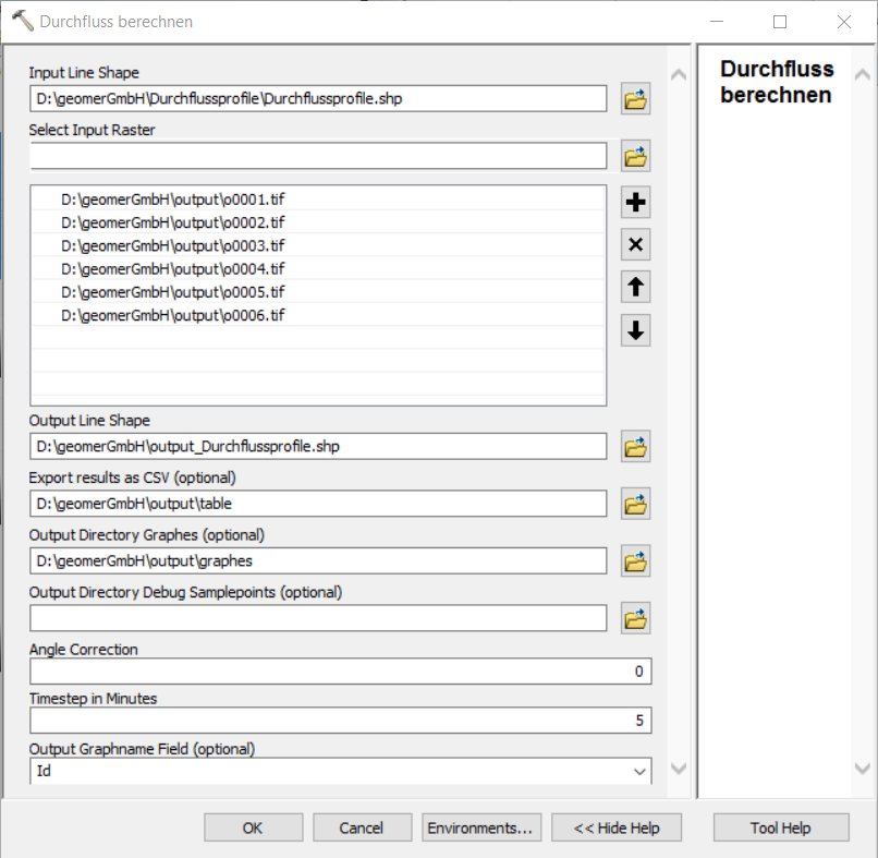
Input Line Shape

A line shapefile is required as input. The runoff is determined along these lines. When digitizing the runoff lines, ensure that there are unambiguous flow directions at this location without strong turbulence or backwater. To ensure that the runoff can be uniquely adressed to a line, the shape requires a column with an unique ID for each line (Output Graphname Field).

Select Input Grid

The calculation of the discharge requires the simulated inundation depths raters in the correct temporal order. Since the tool also needs the corresponding flow velocities and flow directions, which are accessed automatically, the folders output, velocity and direction must have the same structure as they are generated by FloodArea.

Output Line Shape

The calculate discharge tool generates a new shape file with runoff information for every time step in m ³/s. Each time step gets a new column in the attribute table of this shape. Please consider the time step length that you set in the simulation if you want to perform calculations with the individual values.

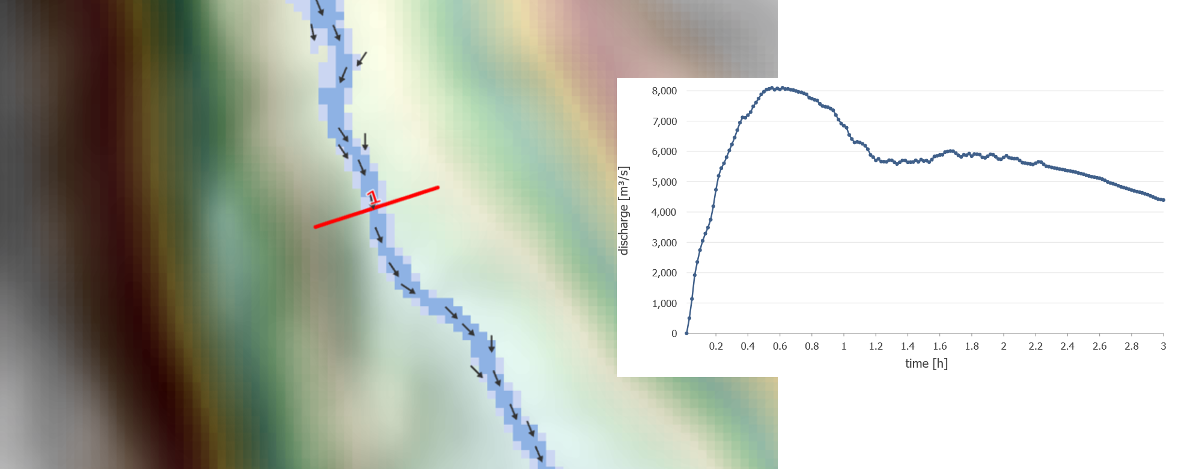
Output Graphs

If a file path is specified in Output Directory Graphs, a flow hydrograph graph is written out for every discharge line, which represents the flow over the simulation time. Using the data in the attribute table of the Output Line Shape, further values can be calculated (e.g. the average and maximum flow rate, sum of flow rate).

Export Results

If a file path is specified here for Output Directory Graphs, the entire results are written out as .csv files.

Further settings

The temporary Samplepoints that are set along the flow lines and through which the tool extracts the data, can also be saved by specifying a path under Output Direcoty Debug Samplepoint. For each time step a shapefile with the flow velocities and directions as well as the water depth or cross-section of the sample points is output. The AngleCorrection changes the flow directions systematically and should be set to 0. The TimeStep corresponds to the time step in which the grids were written out during the simulation (default = 1, if a grid was generated every 60 seconds / 1 minute).

Generate Hydrofiles

If you want to use the point input calculation function, this tool can help you create the hydrograph and coordinate files. To use it, you need a line feature class where the extraction point and injection point are connected by a line. In the Example data folder you’ll find a template that you can adapt to your project (Pay attention to the coordinate system):

When creating pump connections, the digitizing direction of the lines is crucial (starting point = extraction, end point = injection point). Here is an example of an attribute table:

The ID, which is written into the first column of the coordinate file is reassigned based on the order of the FID (first column in attribute table).

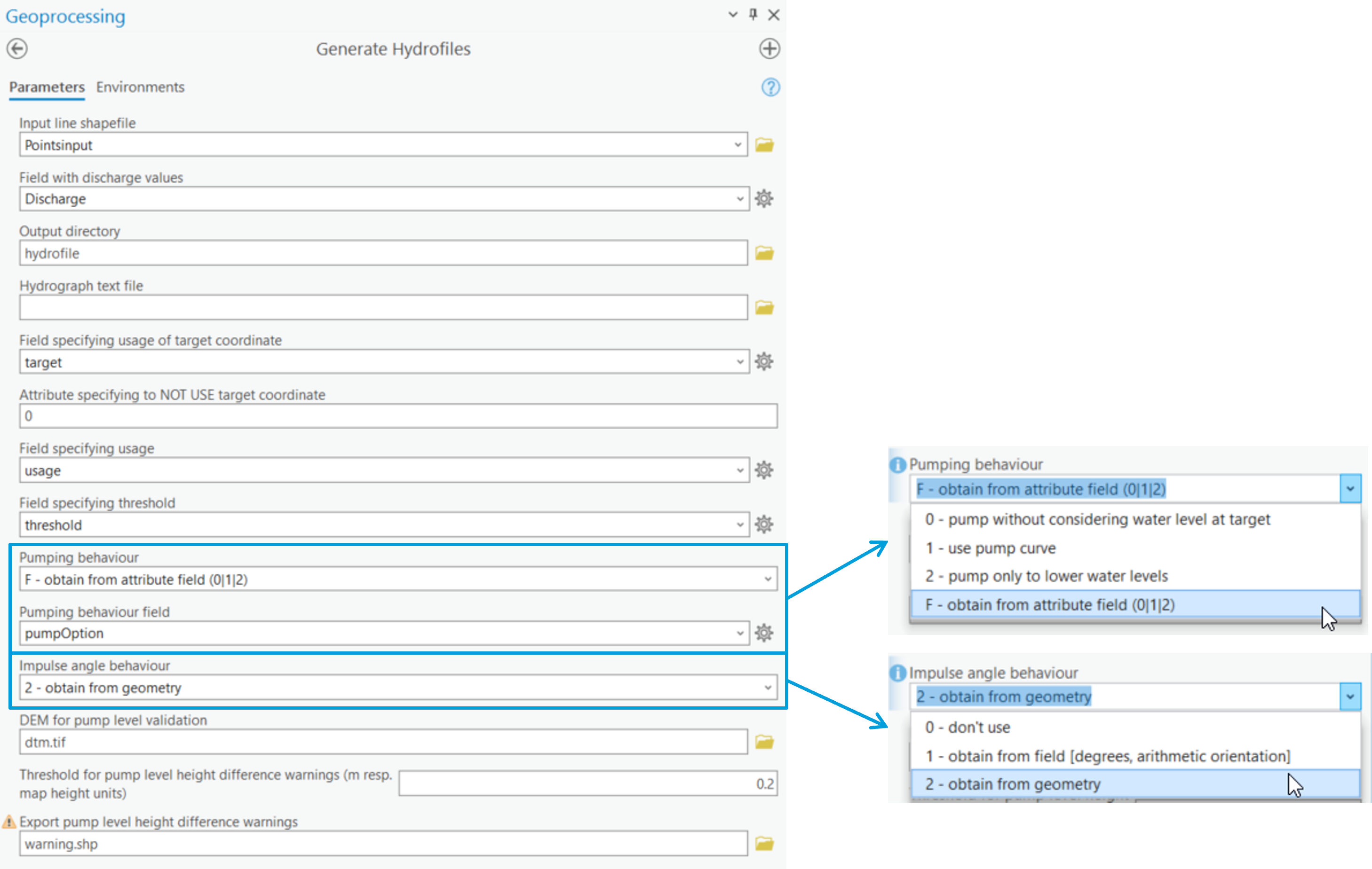
The tool can be used as follows:

Field descriptions:

Attribute column with flow information:

The water quantity to be pumped is in the Discharge column and is written to the Point input hydrograph geschrieben (in m ³/s). If the value is positive, water is pumped out from the initial coordinate (negative value in hydrograph file). If you enter a negative value in the attribute column, injection occurs (positive value in the hydrograph file). Thus, a sign reversal takes place during generation.

Hydrograph text file:

A hydrograph text file can be specified as a template. The time steps (first column in each case) are then adopted. If no rainfall hydrograph is specified, the hydrograph has a time horizon of 8760 hours.

Attribute column with usage information for target coordinate:

Defines whether the extracted water quantity is fed in through the target coordinate (endpoint of the line) or completely removed from the simulation (starting point). This corresponds to the target column in the example feature class. Typically, the value for a pump connection is set to 1 and the value for a point input without target coordinate is set to 0 (default).

Attribute column specifying whether a pump connection should be used:

Distinction of which coordinates water should be pumped to (practical for different scenarios despite one shapefile, definition via 0/1).

Attribute column for threshold value:

Attribute column with minimum water level from which water should be pumped first (specification in cm). One application would be, for example, the inlet structure of a flood retention basin.

Setting the pump behavior:

The switch indicates which pump behavior should be used, i.e., whether the water levels between start and end coordinates should be compared (0, 2) or a pump characteristic curve should be used (1). Options 0, 1, 2 are applied to all line objects in the feature class. For option F, an attribute column in the feature class is used.

Setting the impulse angle:

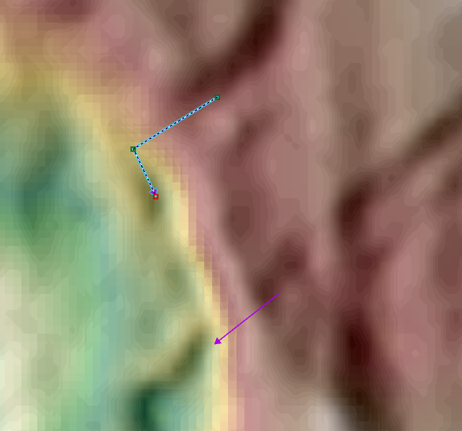
Here it is possible to read out the impulse angle from the geometry of the line. The direction vector of the last segment of a polyline is used. If a connection has only two support points, these are used for the impulse direction. However, you can add additional support points and thus modify the impulse direction. Examples of this are shown in the figure below.

Continue Calculation

If the simulation is terminated prematurely during execution, there are three ways to continue the calculations:

• Backup: If a backup folder exists in the results directory, you can restart the simulation from the history in GIS or the command line (fng.xml in output folder). FloodArea ^HPC 11 automatically accesses the backup. The continuation time step depends on the backup’s save interval.

• Toolbox: Under the optional function Continue Calculation with Existing Grid in the Start FloodArea tool, you can select a flood depth raster from the output folder (e.g., o060.tif). You must also adjust the start time according to the save interval. With an interval of 60 seconds and o060.tif, the start time would be 3600. Note: If you use changing discharge coefficient rasters with the Rainfall calculation option: Beregnung you must select the raster that matches your time step.

• GUI: Continue calculation is done via Calculate Flood Areas and Show Meta Data Info. The necessary settings are taken from the metadata. Of course, pathes from meta date must not been changed meanwhile. There is no possibility to manually change the discharge coefficient raster. A change only occurs when the time step in RainfallSwitchTimes.txt specifies it. The Load Settings button in the main menu reads the settings from the metadata of the selected raster and writes them into the flood calculation dialog. Otherwise, the settings of the last calculation or already specified data are used. On the other hand, the settings of the Additional Settings dialog are always automatically adopted when a continue calculation raster is specified, so that, for example, the same legend and the same storage interval are selected. If a change of the respective settings is desired, these must be made accordingly. The start time of the simulation is automatically set to the simulation time of the continue calculation raster. The start time is interpreted as part of the specified simulation duration.