Calculation Options
Rainfall
With the rainfall option, the terrain is irrigated with a specified precipitation pattern over an area. The runoff coefficients, precipitation amount, and precipitation pattern can vary spatially and temporally.
The simulation of a precipitation, heavy rainfall, or continuous rain event is the typical application of this calculation option. The duration of precipitation can be freely chosen. The proportion of precipitation that leads to runoff can be controlled via one or more runoff coefficient rasters. Through spatially and temporally variable input of rainfall hydrographs and runoff coefficient rasters, real precipitation events can be simulated based on radar data or measured values from ground stations.
Rainstorm data formats
Required data:
Digital terrain model (GeoTIFF)
Runoff coefficient raster (GeoTIFF in float, positive values)
Precipitation hydrograph (.txt)
Optional: File for temporal change of runoff coefficient (.txt)
Optional: Raster for subdivision of the area (GeoTIFF with unsigned integers)
The runoff coefficient raster specifies what proportion of precipitation becomes surface runoff. The precipitation is defined via one (or more) hydrographs in a text file (in m 3/s or mm/h) and applies to the entire area.
The product of the rainfall amount (in the hydrograph) and the value in the respective pixel of the raster results in the effective surface runoff. Spatial variation can be achieved by weighting the rainfall amounts via the raster cells in the runoff coefficient raster.
Areas that should not receive rainfall can contain a ‘0’ or ‘NoData’ in the raster (both are permissible). If the runoff coefficient raster contains the value 0 or NODATA, no water is added in this area. For all other values, the values of the hydrograph (precipitation) are multiplied by the corresponding value of the raster area (runoff coefficient). If the runoff coefficient is 0.5, for example, this means that half of the precipitation runs off on the surface. This allows for weighted input. If no modification of the hydrograph should occur, the runoff coefficient raster must contain the number 1 everywhere. There should be no negative values in the raster.
Note
FloodArea HPC 11 simulates within the extent of the digital terrain model. Runoff into NoData areas is removed from the system. With Release 11.6, buffer edges are no longer necessary.
Rainfall Hydrograph
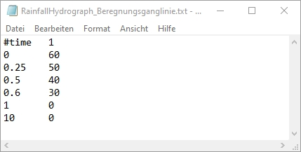
The hydrograph files can be created externally with any editor and must be in text format with the file extension “.txt”. The files must correspond to the following format:
The first line is commented out (´#´) and contains the column names. The first column specifies the time in hours. The period must at least correspond to the simulation duration. An error message appears if, for example, 3 hours are simulated, but the time only goes up to 2 hours. The second column contains the precipitation hydrograph in the unit mm/h (alternatively in m 3/s ). The precipitation amount is specified for each time interval (as a positive number). Linear interpolation is performed between the specified time steps.
For the volume balance, it is important that the hydrograph contains a sufficient amount of precipitation. We use the image of a bucket that is filled by FloodArea with the precipitation of the hydrograph. This bucket of water is only poured into the system (the output rasters) when 1 mm is reached in the hydrograph. This is numerically necessary, in particular to work volume-true between the iteration steps and at the same time to enable a realistic flow field propagation. If the hydrograph always contains only a 1 (i.e., 1 mm/h) for each time step, the threshold value of 1 mm is only reached every 60 minutes and therefore the “bucket” is only tipped into the output raster once per simulation hour.
Conversion between m 3/s or mm/h
In many respects, the two hydrograph options (i.e., point input or rainfall) are similar. If a raster layer with only a single raster cell is specified for areal input, the results are identical to those for a point input at this coordinate. However, the units of the hydrograph must be converted to mm/h. Note that the conversion factors depend on the raster width; the input of the amount specified in the hydrograph takes place per raster cell. Here are some selected values:
The following intensities correspond to an inflow of 1 m 3/s :
This conversion is performed automatically when the inflow rate switch is active in m 3/s . When feeding in m 3/s , the amount of water specified in the hydrograph file is distributed over all raster cells of the rainfall area raster. Cell values in this raster are used as weighting, but the total amount of water supplied is not modified.
Change Runoff Coefficient Over Time
Runoff coefficients change over time during a precipitation event. To represent this, several (any number of) runoff coefficient rasters can be loaded into the simulation one after the other. he temporal exchange of the runoff coefficient rasters is defined in a text file. This can be created externally with any editor and must be in text format with the file extension “.txt”. The file must correspond to the following format:
The first line is commented out (´#´) and contains the column names. The first column specifies the time in seconds (Note: In most other files it is hours).The second column contains the paths to the runoff coefficient rasters. No further columns may be added. Since the first runoff coefficient raster is specified directly, only the subsequent runoff coefficient rasters are specified here.
Vary Precipitation Spatially
To simulate inhomogeneous areal precipitation, several hydrographs can be fed into the simulation. So if you want to simulate a real rain event based on collected data from several precipitation measuring stations, this is easy to implement.
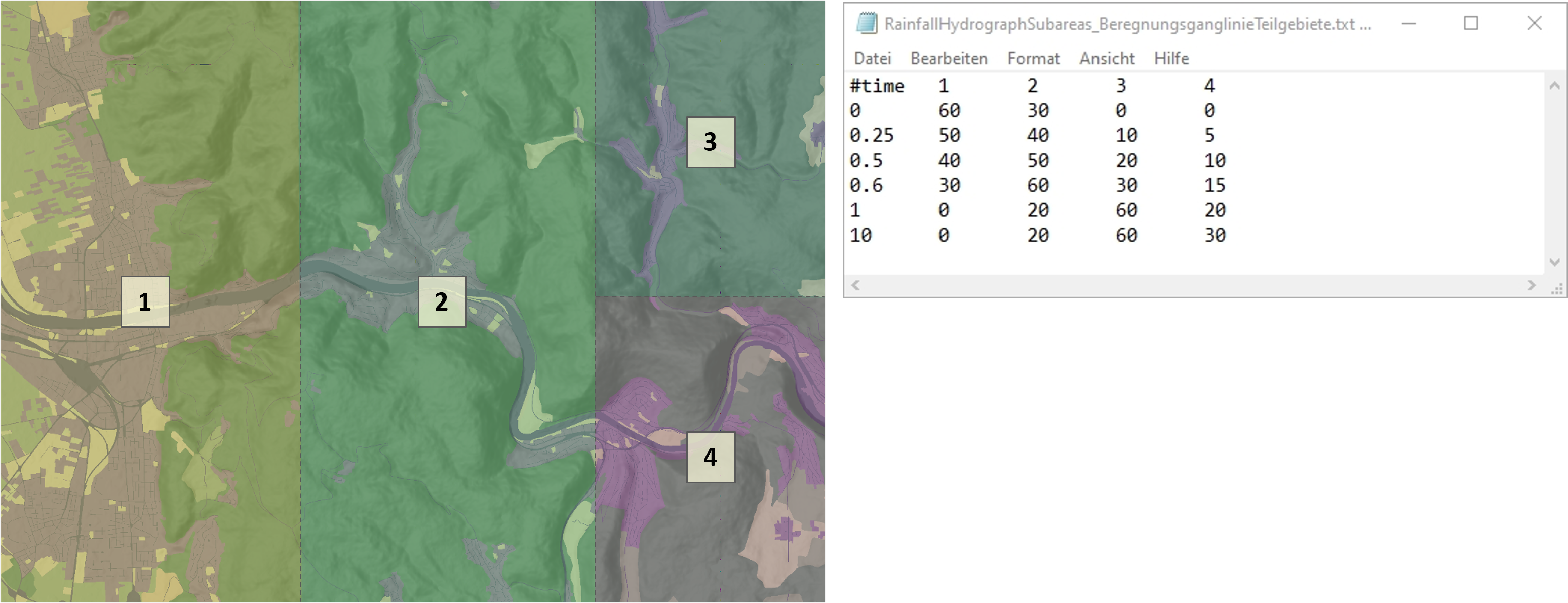
This requires a raster for the spatial subdivision of the rainfall area as well as several hydrographs in the hydrograph file. The raster for the spatial subdivision of the area contains only the ID of the hydrograph with unsigned integers.
The hydrographs are specified analogously to the first hydrograph and written in the subsequent columns. The order of the hydrographs must match the order of the IDs in the raster. Column 1 in the rainfall hydrograph corresponds to the value 1 in the raster, column 2 to the value 2 in the raster, and so on.
The IDs in the subdivision raster and in the hydrograph text file must be identical, start with 1 and follow each other (1, 2, 3, …).
If the numbers do not follow each other, the error message GridValueOutOfRange ~ -119; Subarea rainfall index is out of range. If spatially varying rainfall is activated, but only one hydrograph is entered in the hydrograph file, no error message is issued. Wherever no subarea ID is defined in the raster, the first hydrograph is used (as long as there is a runoff coefficient there).
Rainfall Test Data
The test data for this option are as follows:
DischargeIndex_Abflussbeiwert.tif (4 rasters)
RainstormSubdomains_BeregnungsTeilgebiete.tif
RainfallHydrograph_Beregnungsganglinie.txt
RainfallHydrographSubareas_BeregnungsganglinieTeilgebiete.txt
RainfallSwitchTimes_BeregnungWechselzeitpunkte.txt
Point Input - Pump Connection
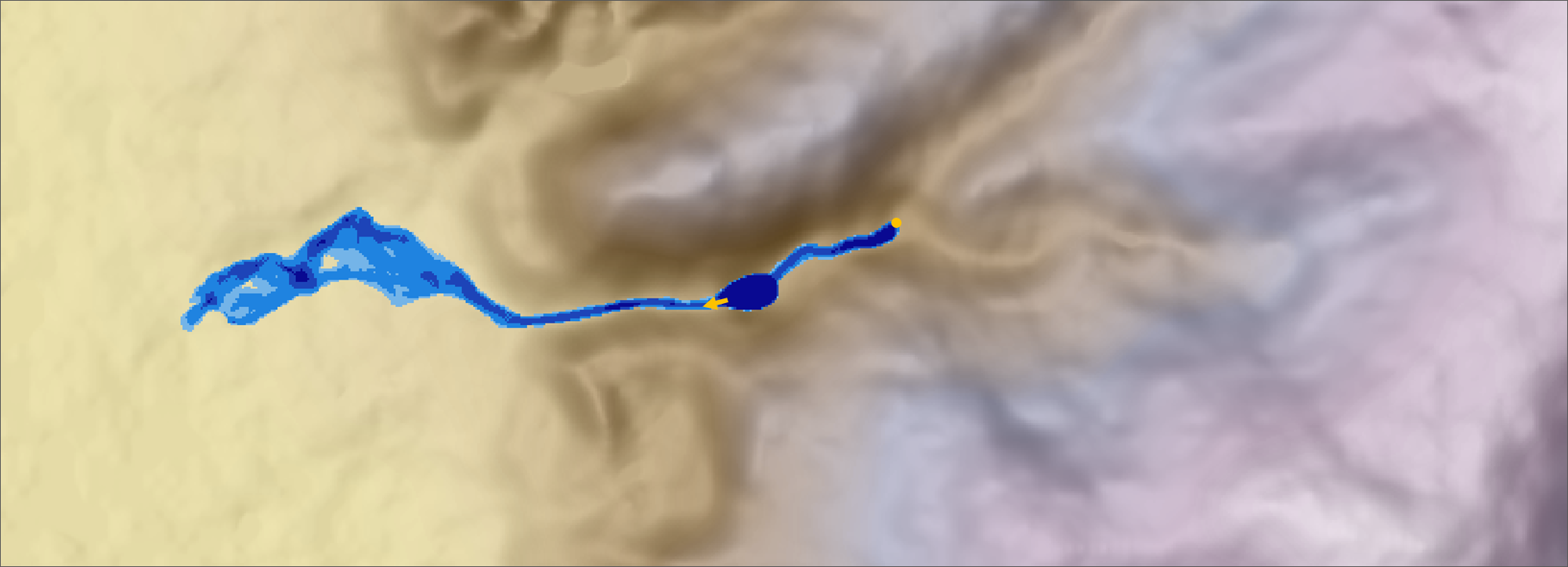
With point input, water is specifically fed into or removed from the model at a coordinate. The pump connection takes water from a start coordinate and feeds the water back in at an end coordinate. The respective amount of water is defined in a hydrograph and can vary over time.
The point input function is frequently used in combination with the rainfall function to depict realistic flow under complex conditions. For example, if small-sized culverts or passages are located under roads, large runoff volumes in reality lead to backwater at the road and only small amounts of water are passed through the culvert. By means of a linear connection, the runoff volume can be taken according to the capacity in front of the road and fed back in behind the road. In ArcGIS, the preparation of the data for this application can be found under the functionality Generate Hydrofiles.
Point Input Data Formats
Required data:
Digital Terrain Model (GeoTIFF)
Hydrographs (.txt)
Coordinates (.txt)
Optional Pump Characteristic Curve (.txt)
The hydrograph defines how much water is removed or fed in at a certain coordinate. The coordinate file defines what should happen at that coordinate. Each column in the hydrograph corresponds to a row in the coordinate file. The structure of the files is explained in the next chapters. Note that with pump connections and water withdrawals, water is only pumped if water is present at the initial coordinate. The actual pumped quantity is written to the file PumpVolume.pum for each time step during the simulation (unit: m 3/s ).
It should also be noted that the input at a coordinate takes place in only one cell and therefore a calculation should only be carried out with reasonable inflow quantities. If the runoff behavior of a very large amount of water is to be modeled (as is the case, for example, with the discharge of a large river), the water should be fed in over several cells, i.e., coordinates. An alternative option is the input of the desired amount of water over a certain area (Calculation Option Rainfall).
The hydrograph and coordinate files can be created externally with any editor and must be in text format with the file extension “.txt”. Alternatively, the Generate Hydrofiles functionality can be used for generation. The use of Generate Hydrofiles is recommended.
Hydrographs
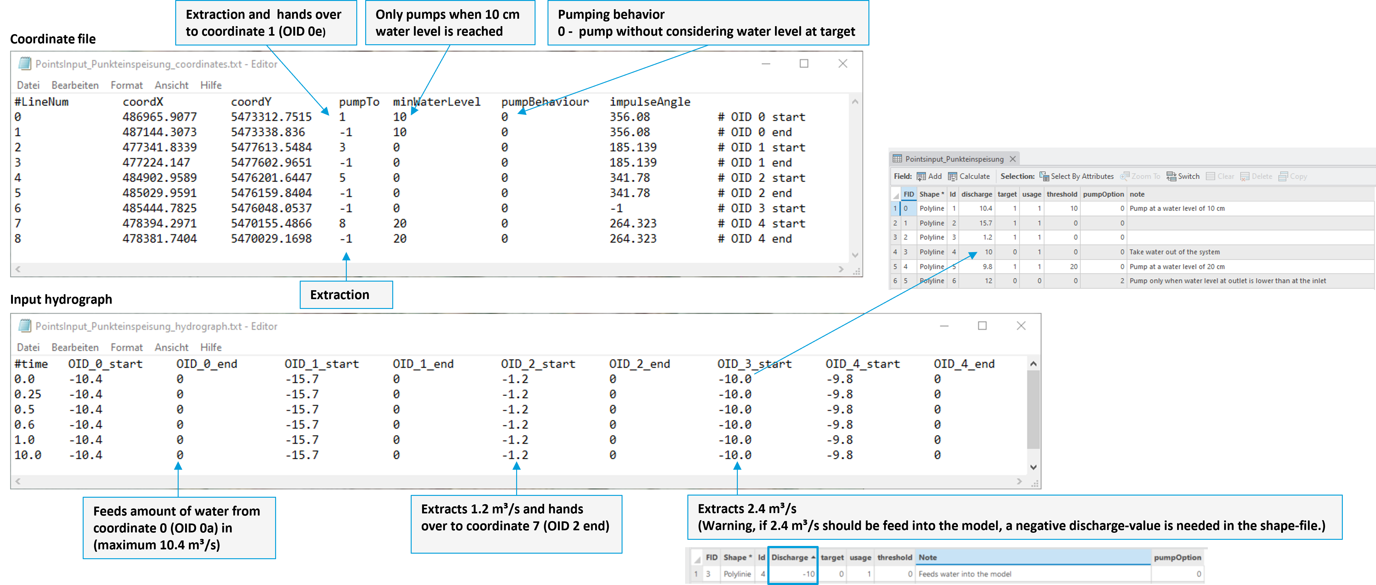
The basic structure of the hydrograph file must correspond to the following format:
The file consists of at least two columns. The first column represents the time intervals (unit: hours). The second and all subsequent columns contain the amount of water. The amount of water is specified for each coordinate in m 3/s and can vary over time. Linear interpolation is performed between the time steps (first row).
Each column (except the first) corresponds to a row with a coordinate pair in the coordinate file. Positive values correspond to inputs, negative values withdraw water. If water is to be transferred from coordinate A to coordinate B, each ID has two columns (e.g., OID_0_start and OID_0_end), as shown in the figure below. 0 is entered in the second column because no further water transfer takes place at this coordinate. If water is only to be removed and fed in at one coordinate, only one column is necessary.
The pumping rates can be modified over time.
Coordinate File
The file with the coordinates must be structured according to the following specifications.
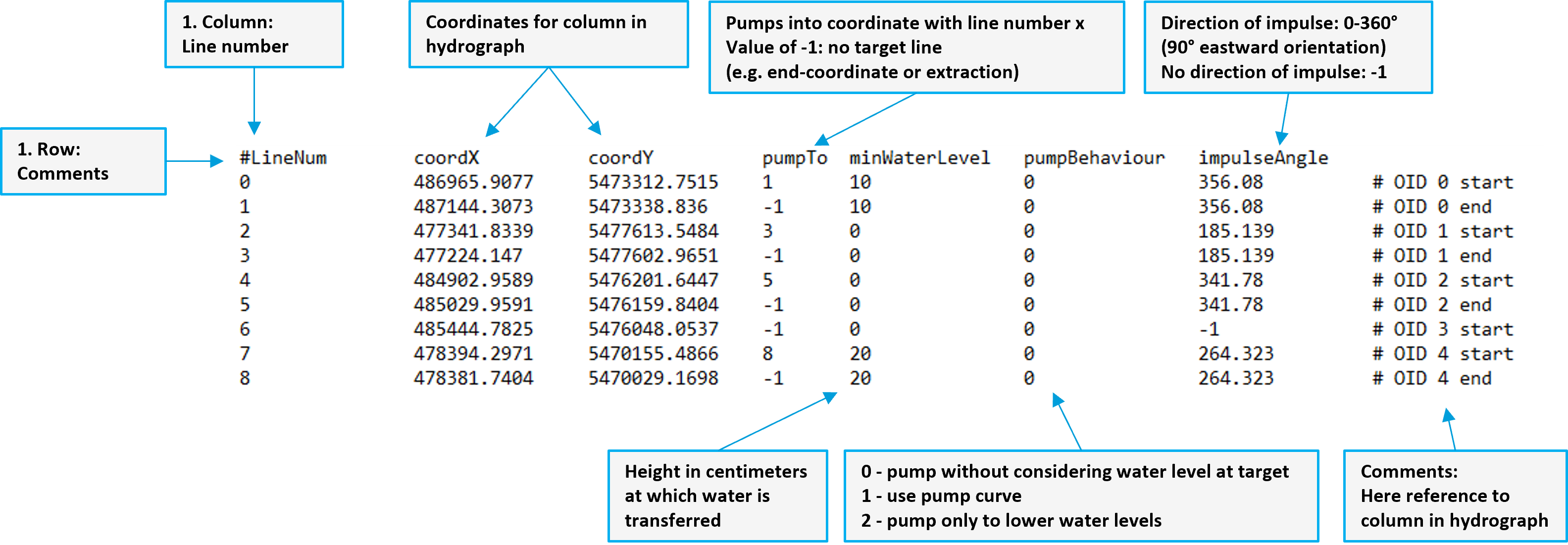
The first line is commented out (´#´) and contains the column names. The first column contains a system-internal ID of the coordinate. This must be unique because it is used by FloodArea HPC 11. Therefore, it should be counted from 0 onwards. Your own IDs or notes can be commented out at the end of the line with a hash (#).
The two subsequent columns contain the coordinates for the input. The fourth column is followed by the ID of the target coordinate into which water taken from the associated withdrawal coordinate is fed back in. The target cell must always be after the withdrawal coordinate in the list because the processing is sequential. If no water is to be taken from a certain cell or if the water taken is to be completely removed from the system, there is no target coordinate into which it is pumped. Therefore, the value -1 must be entered in this row for the target coordinate. The fifth column in the coordinate file (minWaterLevel) contains the minimum water level in the respective cell. The value is given in cm (relative to the surface); other units must be converted accordingly. The minimum water level is always left in the corresponding cell and withdrawal only takes place when this water level is exceeded.
The sixth column is a switch that controls the pumping behavior.
0 The water level at the end coordinate is not taken into account
1 Use a pump characteristic curve
2 The water levels at the start and end coordinates are compared. If it is equal to or higher at the end coordinate, no pumping takes place.
The seventh column controls the impulse direction in which the water should flow at the end coordinate. FloodArea HPC 11 works with the arithmetic direction orientation (rotated 90° to the east). A value of -1 means that no impulse direction should be used.
Warning
For each input point in the coordinate file, there must be a column with discharge values in the hydrograph file. The hydrographs from the file are assigned to the input coordinates of the digitization in their order. If the columns are missing in the file, no inflow is fed in. The same applies to missing input coordinates.
From the combination of the 4th column of the coordinate file (column pumpTo) and the associated hydrograph file, it can only be read whether water is removed from or fed into the model at the coordinate. The inflow or withdrawal quantities are specified by the specified point input hydrograph file.
Some combination possibilities are shown in the following figure:
From these two files, the following information can now be read, for example:
#LineNum 0 and 1: As soon as a water level of 10 cm is reached at coordinate LineNum 0 (OID 0 start), water is removed at coordinate 0 and transferred to coordinate 1 (OID 0 end).
#LineNum 2 and 3: Water is removed at coordinate LineNum 2 (OID 1 start) over the entire hour and fed in at coordinate 3 (OID 1 end).
#LineNum 6: At this coordinate water is removed from or fed into the model at this coordinate over the entire hour.
Special Function: Pump Characteristic Curve
Warning
This function is currently being tested - please ask us before using it!
The pump characteristic curve is a function that originates in water management. It is designed to simulate the pumping capacity of pumping stations and pumps that pump water from lower-lying floodplains or canal network systems into higher-lying river bodies. The lower the height difference that needs to be overcome, the higher the pumping capacity of the pumping station.
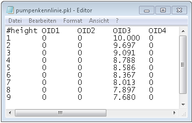
The pump characteristic curve is another text input file, e.g., “Pumpkennline_FloodArea.txt”.
The last column of the coordinate file represents the switch that controls the pumping behavior. If this is set to 1, the pump characteristic curve is used for throughput (pumping capacity) instead of the hydrograph file. The first column of the pump characteristic curve file contains the height differences between withdrawal cell and feed-in cell in decimeters (dm). This column is only for orientation during creation and is ignored by the program. Each line represents one decimeter, so the first line corresponds to a height difference of 1 dm, the last line to a height difference of 100 dm. The file requires a continuous height index, so there must always be exactly 100 entries. Even if certain height ranges are not needed, they must not be deleted but must be set to zero in the pump column. Each subsequent column contains, if required, the characteristic values for the pump used at the corresponding coordinate. In the example, values are only entered for coordinate OID 3.
Point Input Test Data
The test data for this option are as follows:
PointsInput_Punkteinspeisung.shp
PointsInputCoordinates_PunkteinspeisungKoordinaten.txt
PointsInputHydrograph_PunkteinspeisungGanglinie.txt
Water Level
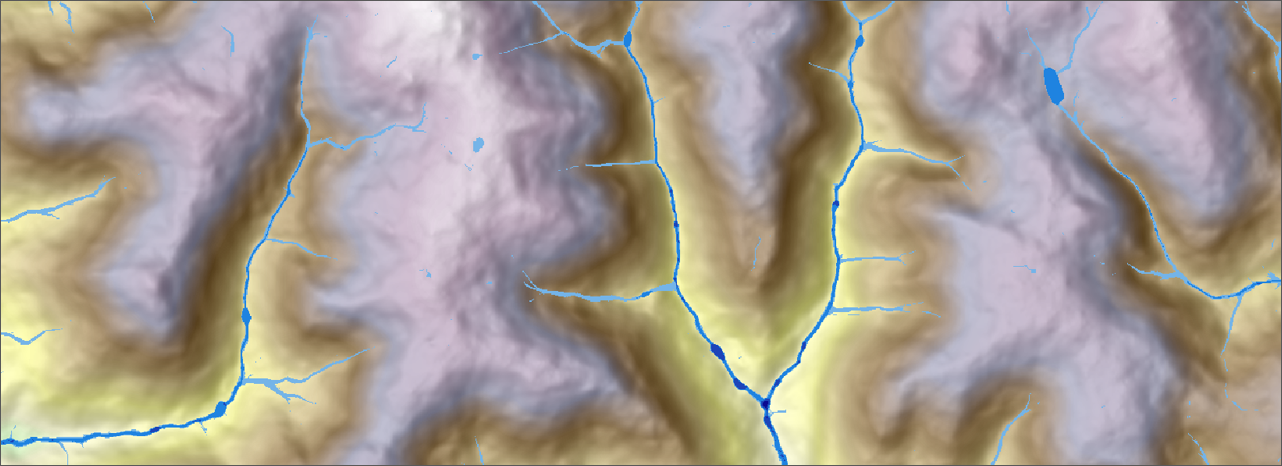
With the water level option, a drainage network forms the starting point for the flood simulation. If the water level in a drainage network rises above the height of the bank, FloodArea HPC 11 simulates the flood area spreading from the water body.
The simulated water level can vary spatially and temporally. The previous function Specify constant height / add to it, with which one could specify an alternative value for the entire drainage network or add a height value, has been replaced by the function temporal modification.
The simulated water level can vary spatially and temporally.
The typical application for the water level option is the simulation of flood events. However, since FloodArea HPC 11 has limitations with respect to channel hydraulics (see chapter Theoretical Principles), we recommend a combined simulation of FloodArea HPC 11 with a 1D model.
Often, various flood marks are available, but there is no complete recording of the flood areas. Here, the flood marks with their absolute height can be specified as water bodies in the model. The surrounding terrain is flooded from these points or lines. Any height differences are interpolated hydraulically in a meaningful way.
Water Level Data Formats
Required data:
Digital Terrain Model (GeoTIFF)
Drainage Network (GeoTIFF)
Optional: Temporal Modification (.txt, unit: cm)
The drainage network raster layer is used to feed water into the model. The initial water level in the drainage network is specified via the pixel values of the raster. The height information of the drainage network can be specified in the following units:
Specification as water level: absolute heights including the height of the DTM (e.g., in m above sea level) or
Specification in flood depth: relative height above the terrain height (e.g., in meters)
In the drainage network raster, there must be no data (NoData) wherever no water level is to be simulated.
Note
At the beginning of each iteration step, the initial drainage network is reset to its initial state. Depending on which flow processes took place in the meantime, water volume is fed into or removed from the model at the affected raster areas.
The water level can vary both spatially and temporally. Spatial variation is achieved via the pixel values of the drainage network raster, while temporal variation requires a hydrograph.
Spatially Varying Water Level
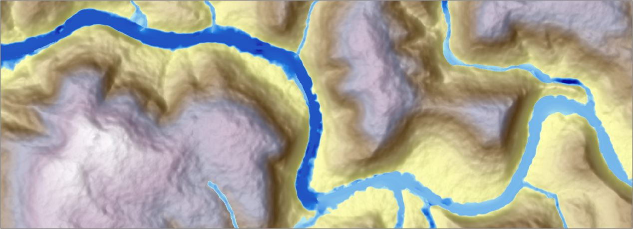
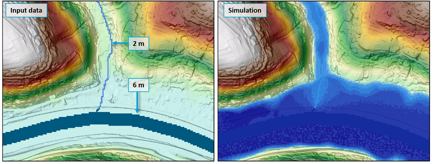
Spatial variation is achieved by assigning different values (heights) to the pixels of the drainage network raster. The following figure shows on the left an initial water level (specification in flood depth), which is 6 m in the main water body and 2 m in the secondary water body. Due to the different initial water levels, the flood extent differs in the result (right).
Temporal Modification of the Water Level
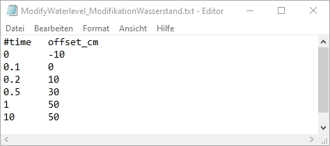
The temporal modification of the water level is given to the simulation via a text file. The first line is commented out (using ´#´) and contains the column names. The first column specifies the time in hours. The second column contains the change in water level in centimeters. The change in water level is specified for each time interval and is added to or subtracted from the initial water level depending on the sign (see figure).
Water Level Test Data
The test data for this option are as follows:
DrainageNetwork_Gewaessernetz_absolute.tif
DrainageNetwork_Gewaessernetz_relative.tif
ModifyWaterlevel_ModifikationWasserstand.txt
Optional Inputs
Flow Roughness
As usual, FloodArea can simulate with a roughness raster. The flow roughness of the land cover is given according to Gauckler-Manning-Strickler (kSt); kSt has the unit m 1/3/s . If no roughness raster is specified, FloodArea uses the value 25 m 1/3/s for the entire area.
Certain roughness values: For unspecified roughness coefficients (NoData), FloodArea HPC 11 uses a default value of 25 m 1/3/s . The value range for flow roughness is >=1 and <=1000. A roughness of “0” is not allowed. The extent of the roughness raster must be identical to that of the DTM.
The roughness rasters should not be larger than the DTM, otherwise errors will occur in the simulation. It is best to intersect the roughness rasters with the DTM before the simulation (Extract by Mask). If the roughness rasters are smaller than the DTM, the roughness 25 is used on the missing areas.
Water Depth-Dependent Roughness
According to the state of research, the roughness values for thin film runoff should be adjusted, especially for vegetated land uses. For example, the buckling of cereals from a certain water level in the field and the resulting smoothing of the surface should be represented in the model. To represent thin film runoff, the user can now specify a second roughness raster. This enables a water depth-dependent change between two roughness rasters.
Required data:
Two roughness rasters (GeoTIFFs with unsigned integers, unit: m 1/3/s )
Threshold value raster (GeoTIFF in floating point, unit of the DTM raster)
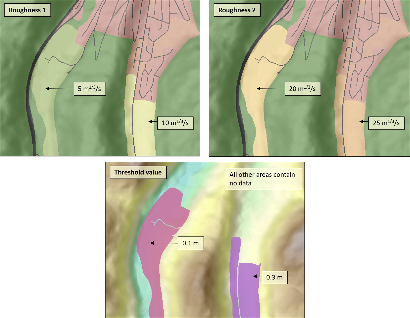
To use this function, a second flow roughness raster is specified and a raster with the threshold values is specified. The first raster contains the roughnesses for the thin film runoff (roughness_1.tiff / Roughness_ras). The second raster contains the roughnesses at higher flood depths (roughness_2.tiff / Roughness2_ras). If FloodArea is started via the command line, the UseVariableRoughness mode must be activated in the fng.xml (true).
Format of the threshold value raster: The raster of the roughness threshold values must be of the data type float and contain the flood depths (unit of the DTM raster) from which the second flow roughness is to be switched to. FloodArea HPC 11 only checks the areas that are also specified in the threshold value raster during the simulation. In the threshold value raster, the pixels in which the flow roughness should not change must be empty (NoData and ‘0’ work).
In addition, two roughness rasters are required, which differ on the areas defined in the raster of the roughness threshold values.
Tip
As an example, in a simulation area, the flow roughness on meadows should change from 5 m 1/3/s to 20m 1/3/s from a water level of 10 cm (based on the assumption that grass buckles from 2 cm flood depth). Accordingly, in the first roughness raster (roughness_1.tif), the meadow must have a value of 5 m 1/3/s and in the second roughness raster (roughness_2.tif), the meadow must have a value of 20m 1/3/s . In the Roughness Threshold Value raster, all meadows are given a value of 0.1 m. On arable land, on the other hand, the roughness should not change until a water level of 0.3 m and change from 10 to 25 m 1/3/s . The pixels in which the roughness should not change have no threshold value (NoData or ‘0’).
Roughness Interpolation
In Baden-Württemberg (Germany), there are special requirements for the roughness approach within the framework of municipal heavy rain risk management. According to the guideline, the roughness should be interpolated depending on the depth:
Up to a flood depth of 2 cm, a “thin film” roughness is used,
From 10 cm, the roughness value from the literature is used,
In between, linear interpolation is used.
Under AdditionalOptions, the line <UseInterpolatedRoughness>true<UseInterpolatedRoughness> must be inserted (pay attention to the order of the parameters). In addition, two roughness rasters must be specified for the paths - but no threshold value raster. The two roughness rasters each specify the values between which interpolation is to take place. Optionally, limits can be set that represent the limits of the interpolation (in centimeters):
UseInterpolationLowerLimit specifies the lower limit of the interpolation,
UseInterpolationUpperLimit specifies the upper limit of the interpolation.
If no Lower or Upper Limit is specified, 0.02 is automatically used as the Lower Limit and 0.1 as the Upper Limit, the unit is the same of the DTM raster
Tip
A meadow receives roughness 5 in the first roughness raster and roughness 20 in the second roughness raster. The user does not enter any values for the Lower Limit or the Upper Limit. On this meadow, the roughness 5 m 1/3/s is then used for a water level up to 0.02 and the roughness 20 m 1/3/s from a water level of 0.1. For water levels between 0.02 and 0.1 , linear interpolation between 5 and 20 m 1/3/s is used.
Negative limits are not allowed. In this case, you will find the following error message in the log file: “For roughness interpolation, either upper limit or lower limit is negative, which is not allowed. Please correct the values in the AdditionalOptions section.”
Roughness Values for Download
Due to the large number of land use types and their various roughness values, we provide you with two lists of assignments as examples. The roughness values in both lists correspond to the guidelines for municipal heavy rain risk management in Baden-Württemberg (Link LUBW).
One list provides a single value for each land use class. The other list has two columns for interpolating the depth-dependent roughness. The object numbers come from the official Alkis dataset. Thus, the list can be used as a lookup table directly in GIS for German projects.
Here you can download the two Excel lists: Link geomer
Infiltration
Equivalent to the Rainfall function, in which water is fed into the model over an area, water can be removed from the simulation over an area. The infiltration rate can vary spatially and temporally.
Required data:
Infiltrationsraster (GeoTIFF with unsigned integers)
Infiltrations-Ganglinie (.txt)
Optional: Raster for subdivision of infiltration areas (unsigned GeoTIFF)
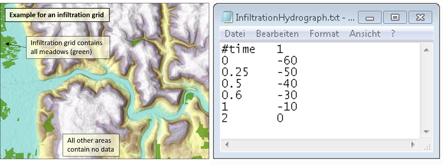
The infiltration hydrograph file can be created externally with any editor and must be in text format with the file extension “.txt”. The files must correspond to the following format:
In the hydrograph, the infiltration quantity is given equivalent to the precipitation hydrograph in mm/h. However, the quantity is given in negative numbers so that the corresponding quantity is removed at the raster cell.
The spatial variation can be achieved by weighting the infiltration quantities over the raster cells in the infiltration raster. The product of the infiltration rate (in the hydrograph) and the value in the respective pixel of the raster gives the effective infiltration. Areas on which no infiltration is to take place can contain a ‘0’ or ‘NoData’ in the raster (both are permissible).
If there is not enough water available, the cell is emptied and the remaining quantity to be removed is ignored. The infiltration quantity is linearly interpolated between the time points.
It is possible to vary the infiltration areas spatially. This is done similarly to the subdivision of rainfall areas by adding additional columns in the hydrograph file and defining the different infiltration areas in a separate raster.
Sewer Network Model
cePipe - Sewer Network Modelling
cePipe is a software product from ce-tools - Civil Engineering Tools.
cePipe is a software for the design and modeling of free-surface channels and pressure pipe networks. It is used in the fields of wastewater disposal and water supply in urban water management. The software is easy to use and quickly ready for use with a short training. cePipe is not a replacement for CAD programs or geographic information systems, but rather an extension for both systems. The program is to be seen as a supplement for the field of activity of a hydraulic engineer.
Further information can be found at https://ce-tools.at/index.php/produkte/cepipe FIf you have any questions about the software, please contact Civil Engineering Tools at Office@ce-tools.at.
Coupling with FloodArea HPC 11
The hydronumeric coupling of the 1D sewer network model cePipe with the 2D hydraulic surface runoff simulation of FloodArea HPC 11 takes place via bidirectional coupling. The data exchange takes place once per minute of the simulation time. In the fng.xml, there is the option to change the simulation time to seconds.
For the coupled simulation, cePipe and FloodArea HPC 11 must be installed on the same computer.
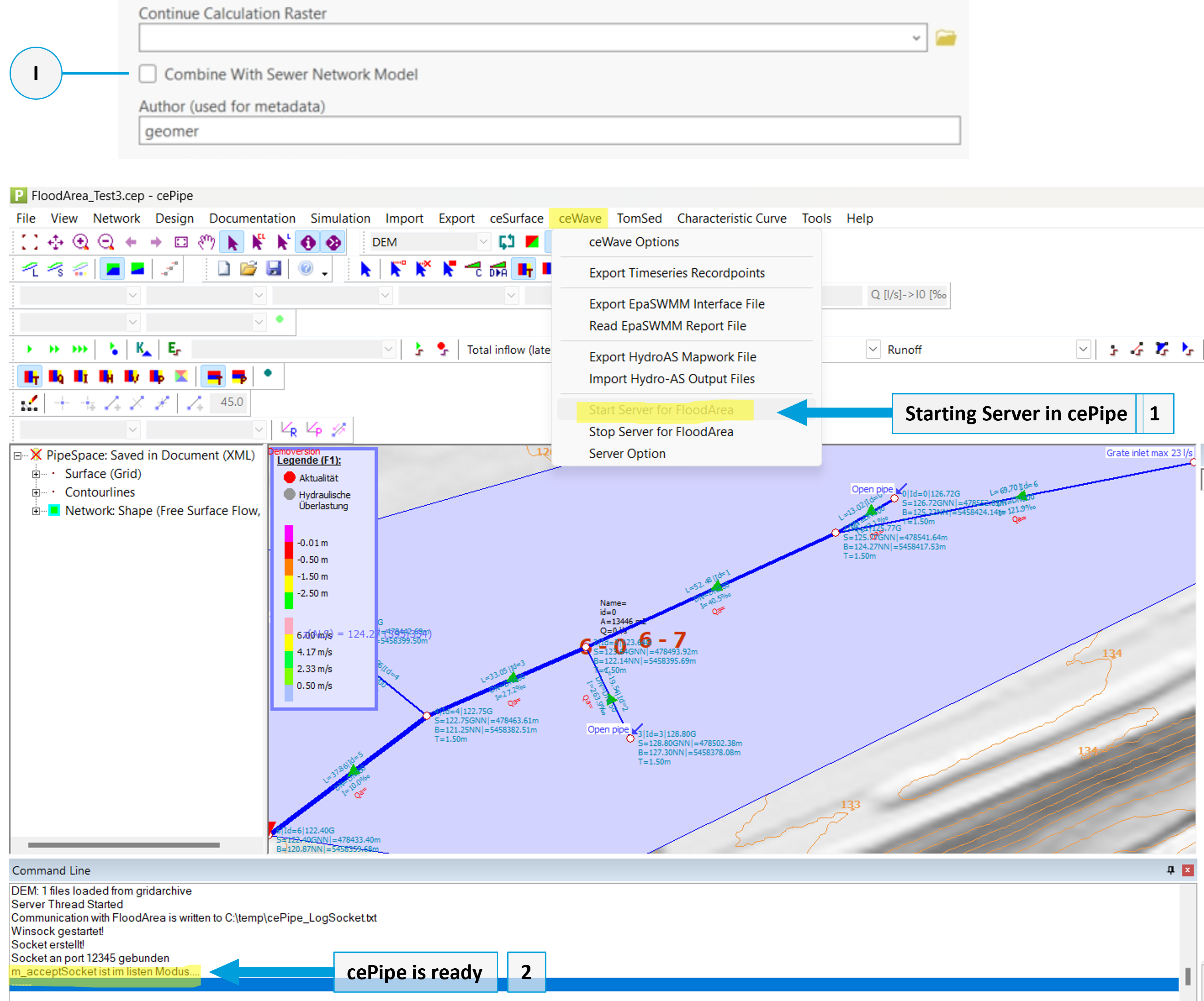
Please refer to the corresponding manual for data preparation for cePipe. The server must be started for the simulation:
1: under Help press Start Server
2: in the Command Line of cePipe you can now see whether the server is ready. If it is, the line …is in listen mode… appears
The simulation starts in both programs as soon as the FloodArea simulation is started. The following figure shows how the sewer network model is activated when FloodArea HPC 11 is started via the GUI and via the fng.xml. In the GUI, only the checkbox Activate coupling with sewer network model must be activated. In the fng.xml, the line “<CombineWithSewerNetworkModel>true</CombineWithSewerNetworkModel>” is inserted under CalculationOption according to the specification by the Config.xsd.
If FloodArea is started via the toolbox, only the checkbox Combine With Sewer Network Model is activated. Then FloodArea HPC 11 can be started as usual.
