Theoretical Principles of FloodArea HPC 11
Fields of Application
FloodArea HPC 11 calculates flood areas based on:
A watercourse with a specified water level, where water overflows the banks and spreads into the surrounding area (fluvial flooding). The Water Level can vary spatially (e.g. along the course of a river) and temporally.
A point input, which adds or removes water at specific coordinates in the model. The inflow amounts of the Point Input are variable in time and space and can also be defined depending on water level.
A rainfall event, where water is added over a larger area. The Rainfall can be spatially divided and carried out with different precipitation hydrographs. The runoff coefficient of the study area can be changed over the course of the simulation.
These three calculation options can be freely combined. The calculation results are output as GeoTIFFs at user-defined time intervals. This allows the temporal sequence of flooding to be traced in as much detail as required. The results can be output or displayed either in absolute elevation values or as flood depth (height difference to the surface). If necessary, current flow directions and flow velocities can also be output for each time interval.
The simulation can be specified in detail by providing additional parameters (Optional Functions). In order to better adapt flow velocities to reality, supplementary roughness coefficients, or roughness, can be specified as a raster. The roughness can be automatically increased or decreased depending on flood depth. This enables realistic representation of flow behavior in dense vegetation.
Calculation Principles
The calculation of flood areas is based on a hydrodynamic approach. The 8 neighbors of a raster cell are considered, from which 32 flow directions are derived. The discharge volume to the neighbors is calculated using the Manning-Strickler flow formula:
where \(r_{hy}^{\frac{2}{3}}\) is the hydraulic radius and \(I^{\frac{1}{2}}\) is the slope.
Detailed tables are available for the \(k_{St}\) values (roughness), which is a clear advantage of this flow formula compared to similar ones. Since roughness has a linear effect on flow velocity ( \(V\) ) an accurate estimation is crucial for the quality of simulation results.
The flow depth results from the difference between the water level and the maximum terrain height along the flow path in the corresponding iteration interval:
In each iteration step, the slope of the water level is recalculated and the water level line in the direction of the steepest slope is used for the slope specification in the Manning-Strickler formula.
Note
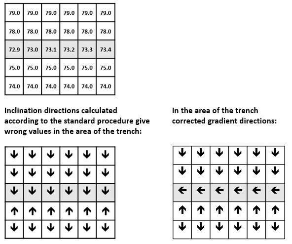
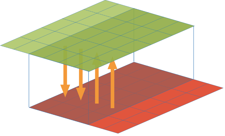
This calculation of slope and aspect can fail in special cases. For 1-pixel wide linear elements, the slope may sometimes be calculated transverse to the channel if the channel bottom has a lower gradient than the surroundings. To avoid such errors, the result is checked for plausibility by comparing the height value of the respective central raster cell with the one in the slope direction. If the cell in the slope direction has higher values, the lowest value from the 8-neighbor environment is sought and the slope is derived directly from the height difference.
The following example shows height values of an exemplary original elevation model with a channel. The slope of the channel here is less than the slope of the terrain (image below).
The calculated flow velocity is multiplied by the flow cross-section and the iteration interval to determine the exchange volume for the current calculation step. As the Manning-Strickler flow formula is only valid for normal flow (i.e., friction loss equals gain in potential energy), sometimes too high flow velocities are calculated outside the validity range (e.g., during acceleration). Therefore, the calculated flow velocities are checked against the limit criterion:
\(V = \sqrt{g \cdot h}\) (velocity of propagation of interfering waves)
Velocities that are too high are reduced accordingly.
Along with the volumes, the velocity vectors are also transferred. These are added and used as the base velocity for the following iteration interval. To determine the respective flow velocity, the weighted mean is calculated from the current velocity calculation and the result of the vector addition. This velocity transfer minimizes sudden flow changes or flow reversal processes and simulates inertia effects in a simplified way.
Computing performance
FloodArea HPC 11 is parallelized - during simulation, the area is divided into tiles (Tiling) and these tiles are distributed across the processor cores of the computer.
The tiles overlap by 4 pixels at the edges in order to synchronize the simulated runoff at the tile boundaries. In older versions, the tiles only overlapped by 3 pixels - the increase in overlap pixels has led to improved synchronization and higher accuracy of the volume balance. The division of the area across the computing cores leads to optimal use of processing power, regardless of the number of cores. The preprocessing of input data, which previously ran separately via Python scripts, has now been included in the core using C++. This has significantly simplified the calculation start and reduced the time required. The simulation time depends on the individual hardware, but tests on different computers showed reductions in calculation times by a factor of 2 to 3 compared to FloodArea HPC 10.3. Tests carried out as part of a academic research project showed speed increases of up to a factor of 4. FloodArea HPC 11 also exhibits greater stability of the computing time in relation to the size and, in particular, the shape of the simulation area (proportion of NoData, fit of the tiles, etc.) than FloodArea HPC 10.3.
Limitations
Volume Balance with Small Water Quantities
It should be noted that FloodArea is designed for water quantities typical of river floods or heavy rainfall. Flow processes (both in reality and in the model) only begin from a few 1/10 millimeters. FloodArea calculates internally with values of 1/100 mm. E

