Basics of FloodArea
Fields of application
FloodArea HPC 11 calculates flood areas based on three options:
A watercourse with a given water level, so that the water flows over the banks and is inundating the surrounding area (flooding). The water level can vary spatially (e.g. along a river course) and temporally.
A point input, where water is taken out or given into the model at specified coordinates. The volumes of the point input are variable in time and space and can also be dependent on water level.
A rainfall event with water that is supplied over larger areas. This option can be used for the simutlation of precipitation events. The Rainfall can be spatially divided and carried out with different precipitation hydrographs. The runoff coefficient of the investigated area can be changed over the time of the simulation.
These three calculation options can be freely combined. The calculation results are GeoTIFFs rasters in a time interval freely selectable by the user. Due to the temporal sequence of the resultes, the flooding can be traced back in any detail. The result output units can be in absolute heights or in flood depth (height difference to the surface). If required, the current flow directions and flow velocities can also be written for each time interval.
The simulation can be specified in detail by specifying additional parameters (Optional functions). In order to optimize the adaption of the flow velocities to reality, Roughness coefficient, in the following regarded as roughness, must be given in the form of a grid. The roughness can be increased or decreased automatically depending on the depth of flooding or by means of a switch. This allows a more realistic representation of the flow behaviour in dense vegetation.
Principles of the calculation method
The calculation of the floodplains is based on a hydrodynamic approach.
Every grid cell has eight neighbours and each of them is going to be considered for calculation in any case. The discharge volume from a grid cell to its neighbours is calculated using the Manning-Strickler flow formula:
where \(r_{hy}^{\frac{2}{3}}\) is the hydraulic radius and \(I^{\frac{1}{2}}\) is the slope.
Detailed tables are available for the \(k_{St}\) values (roughness), which is a clear advantage of this flow formula over comparable ones. Since the roughness is linearly integrated into the flow velocity ( \(V\) ), the best possible estimation is decisive for the quality of the simulation results.
The flow depth results from the difference between water level and maximum ground level along the flow path in the corresponding iteration interval:
In each iteration step, the slope of the water level is recalculated and the water level line in the direction of the largest slope is used for the slope specification in the Manning-Strickler formula.
remark
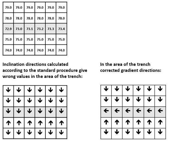
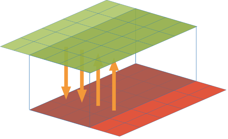
However, this calculation of slope and exposure fails in special cases.In the case of 1 pixel wide linear elements, the slope may be partially transverse to the trench so that the trench bottom is less inclined than the surroundings.
In order to avoid such errors, the result is checked for plausibility by comparing the height value of the respective central grid cell with the one located in the direction of inclination. If the cell has a higher height values in the inclination direction, the lowest value from the 8-neighbour environment is searched for and the inclination is derived directly from the height difference.
The following example shows height values of an exemplary original height model with a trench (gray parcels). Here the slope of the trench is smaller than the slope of the terrain (picture below).
The calculated flow velocity is multiplied by the flow cross section, the iteration interval and the results in the exchange quantity from the current calculation step. The Manning-Strickler flow formula is only valid for normal flow (i.e. friction loss equals the gain in local energy). This sometimes results in too high flow velocities, when calculated outside the range of validity (e.g. during acceleration). Therefore, the calculated flow velocities are checked to see whether they meet the limit criterion
\(V = \sqrt{g \cdot h}\) (velocity of propagation of interfering waves).
Velocities that are too high are reduced accordingly.
Water volumes and the speed vectors are transferred at the same time. Three speed vectors are added and used as the basic speed for the following iteration interval. To determine the respective flow velocity, the arithmetic mean is formed from the current velocity calculation and the result of the vector addition. This velocity transfer minimizes sudden flow changes or flow reversal processes and simulates inertia effects in a simplified way.
Computing performance
FloodArea HPC 11 is parallelized - the area of intrest is divided into tiles during the simulation (tiling) and the tiles are distributed over the pyhsical processor cores of the computing computer.
The tiles are overlaping at the edges by 4 pixels to synchronize the simulated runoff at the edges of the tiles. In older versions, the tiles overlapped only by 3 pixels - The increase of the overlapping pixels has improved the synchronization and made the volume balance more accurate. The division of the area between the operating cores leads to an optimal use of the proccessing power, independent of the number of cores.
The preprocessing of the input data, which previously ran separately via Python scripts, is now implemented in the core with C++. This simplified the start of the calculation and shortened the require time significantly. Intensive benchmark tests show, that simulation time was shortened by a factor of 2 to 3 compared to FloodArea HPC 10.3, due to these improvements.
During tests for research projects, speed increases of up to a factor of 4 were achieved. FloodArea HPC 11 also shows a higher stability of the computing time compared to the size and especially the shape of the simulation area (share of NoData, fit of tiles etc.) on, as FloodArea HPC 10.3.
Limitations
Volume balance with low water volumes
It should be noted that FloodArea HPC 11 is made for river flooding or heavy rain. FloodArea calculates internally with integer values of 1/100 mm and water quantities from 0.02 mm are written to the output. Earlier versions of FloodArea had only a threshold value of 1 mm. However, this means that the water balance is not appropriate for precipitation below the wetting loss and volume losses dealing with low precipitation amounts becomes relatively smaller with larger amounts of precipitation. With normal heavy rain events, the volume loss has a maximum of 1-2%. Flow processes start (real and in the model) only from a few 1/10th of a millimetre, the exchange quantity between the grid cells must be at least 1/100 mm (smallest possible value) in the model.
Observation of peripheral areas
The periphery of the simulation area can lead to problems, because no information about the area beyond the examined area is available. FloodArea HPC 11 assumes here a continuation of the slope of the water surface beyond the edge of the terrain model. Based on this assumption, water from the model is taken according to the calculated outflow volumes. Thus there is no unrealistic accumulation of the discharge volumes at the edge of the terrain model.

