Optional entries
Roughness
As usual, FloodArea can simulate with one roughness grid. The flow roughness of the land cover is given according to Gauckler-Manning-Strickler (k St ); k St has the unit m 1/3/s. If no roughness grid is specified, FloodArea uses the value 25 m 1/3/s for the entire area.
Certain roughness values: For unspecified roughness coefficients (NoData), FloodArea HPC 11 uses a default value of 25 m 1/3/s. A roughness of „0“ is not allowed. A roughness of „10000“ results in a flow blockage.
The roughness grids shouldn’t be larger than the DTM, otherwise errors will occur in the simulation. It is best to cut the roughness grids with the DTM before the simulation (Extract by Mask). If the roughness grids are smaller than the DTM, roughness 25 is used on the missing surfaces.
Water depth-dependent roughness
According to the state of research, the roughness values for thin film runoff should be adjusted, especially for land uses with vegetation. For example, the buckling of cereals above a certain water level in the field and the resulting smoothing of the surface should be represented in the model. To represent thin-film runoff, the user can now specify a second roughness grid. This enables a water depth-dependent change between two roughness grids.
Required is:
Two Roughness-grid’s (GeoTIFF’s with unsigned integers, unit: m 1/3/s)
Roughness-Threshold-grid (GeoTIFF in floating point, unit: m)
To use this function, a second flow roughness grid is specified and a grid with the threshold values is specified. The first grid contains the roughness for the thin film runoff (Roughness / Roughness_ras). The second grid contains the roughness for higher flooding depth (Roughness2 / Roughness2_ras). If FloodArea is started via the command line, the UseVariableRoughness mode must be activated in the fng.xml.
Format of the Roughness-Threshold grid: The grid of roughness threshold values have to be of the data type float and contain the flooding depths (in meters) for switch to the second flow roughness. FloodArea HPC 11 checks during the simulation only the areas which are specified in the threshold grid. The pixels where the flow roughness should not change have to be empty (NoData and ‚0‘ work).
In addition, two roughness grids are required, which differ at the areas defined in the roughness threshold grid.
example
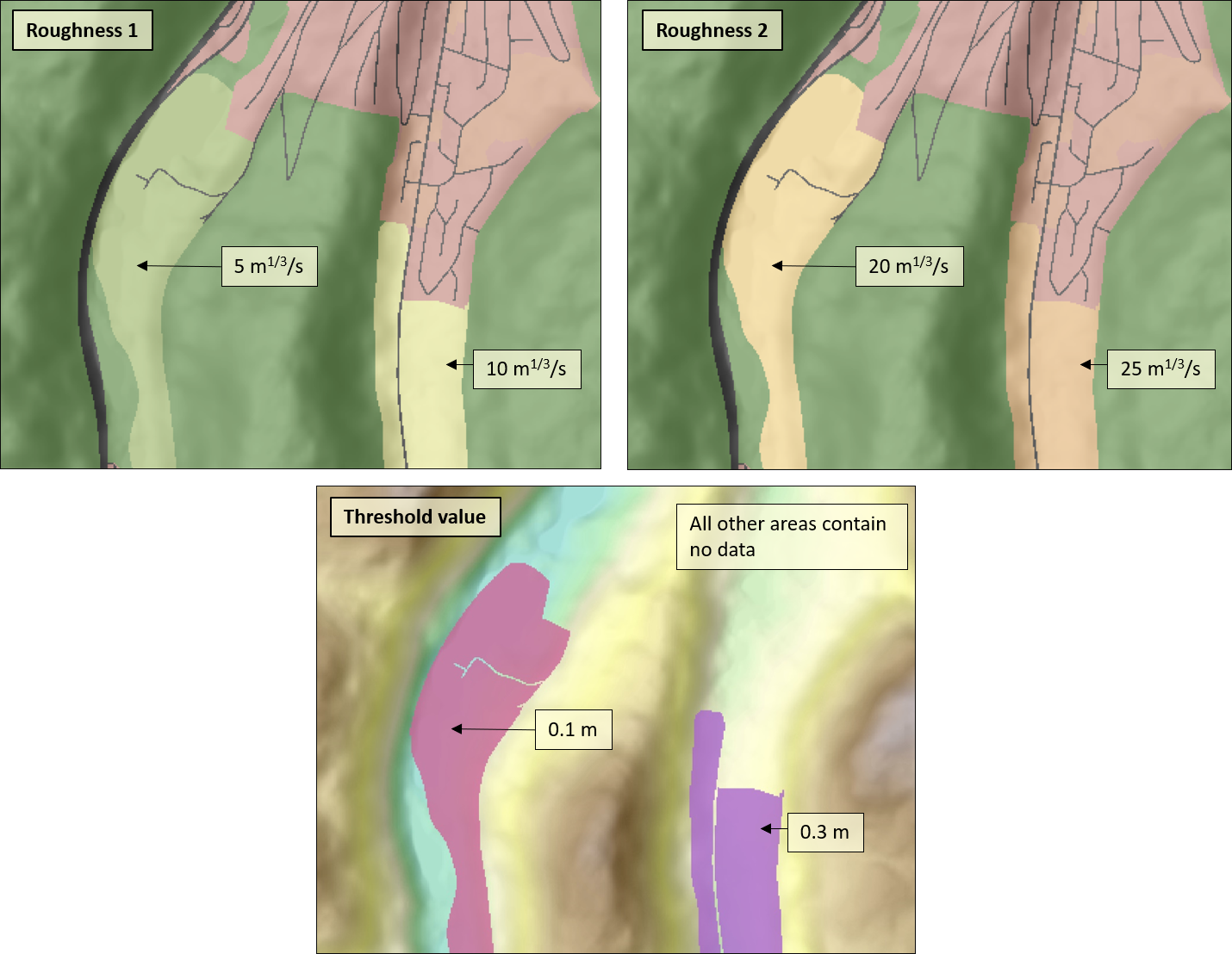
In a simulation area the flow roughness on meadows from a water level of 10 cm should change from 5 m 1/3/s (roughness 1) to 20 m 1/3/s (roughness 2) (based on the assumption that grass bends from 5 cm flooding depth). Accordingly, in the grid flow roughness the meadow must have a value of 5 m 1/3/s and in the Grid second roughness the meadow have a value of 20 m 1/3/s. In the grid Roughness threshold value all meadows are given a value of 0.1 m. On arable land, on the other hand, the roughness should not change until the water level reaches 30 cm, changing from 10 to 25 m 1/3/s. The pixels in which the roughness should not change have no threshold value (NoData or ‚0‘).
Roughness-Interpolation
In Baden-Württemberg (Germany) there are special requirements in the context of municipal heavy rainfall risk management for the roughness approach. According to the guideline, the roughness should be interpolated depending on depth:
Up to a flooding depth of 2 cm, a „thin film“ roughness is used,
From 10 cm, the roughness value from the literature is used,
In between, linear interpolation is used.
This function can be used with FloodArea, but only by adjusting the fng.xml and starting it from the command line (the function is neither implemented in the toolbox nor in the GUI). The following figure shows the fng.xml.
Under AdditionalOptions the line <UseInterpolatedRoughness>true<UseInterpolatedRoughness> must be inserted (pay attention to the order of the parameters). In addition, two roughness grids have to be specified for the paths - but no threshold grid. The two roughness grids specify the values between which interpolation is to take place. Optional limits can be specified to represent the limits of the interpolation (in centimetres):
<UseInterpolationLowerLimit> specifies the lower limit of the interpolation,
<UseInterpolationUpperLimit> indicates the upper limit of interpolation.
If no lower or upper limit is specified, 0.02 m is automatically used as the lower limit and 0.1 m as the upper limit.
example
A meadow receives roughness 5 in the first roughness grid and roughness 20 in the second roughness grid. The user does not enter any values for the Lower Limit or the Upper Limit. In this way, for a water level up to 0.02 m, the roughness 5 m 1/3/s is used and from a water level of 0.1 m the roughness 20 m 1/3/s. For water levels between 2 and 10 cm, linear interpolation between 5 and 20 m 1/3/s is used.
Negative limits are not allowed. In this case you will find the following error message in the log file: „For roughness interpolation, either upper limit or lower limit is negative, which is not allowed. Please provide a positive value.“
Infiltration
Equivalent to the function Rainstorm, in which water is fed into the model over an area, water can be removed from the simulation over an area. The infiltration rate can vary spatially and temporally.
Required:
Infiltration grid (GeoTIFF with unsigned integers).
Infiltration hydrograph (.txt).
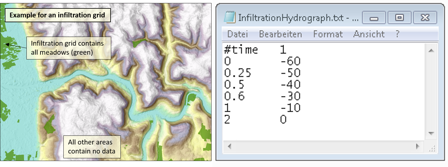
The infiltration hydrograph file can be generated externally with any editor and must be in text format with the file extension „.txt“. The files must conform to the following format:
In the hydrograph, the infiltration quantity is given equivalent to the precipitation hydrograph in mm/h. However, the amount is given in negative numbers so that the corresponding amount is taken at the grid cell. The infiltration quantity is linearly interpolated between the time points.
The spatial variation can be achieved by weighting the infiltration amounts over the grid cells in the infiltration grid. The product of the infiltration rate (in the hydrograph) and the value in the respective pixel of the raster gives the effective infiltration. Areas on which infiltration is not to take place can contain a ‚0‘ or ‚NoData‘ in the raster (both are permissible).
If there is not enough water, the cell is emptied and the remaining amount to be extracted is ignored.
Continue Calculation
A simulation can be continued via a flooding depth grid. The desired flooding depth grid is specified when starting FloodArea HPC 11.
The continue calculation can be done in four ways: GUI - Calculate Flood Areas, GUI - Display simulation info, Toolbox and start via command line.
GUI
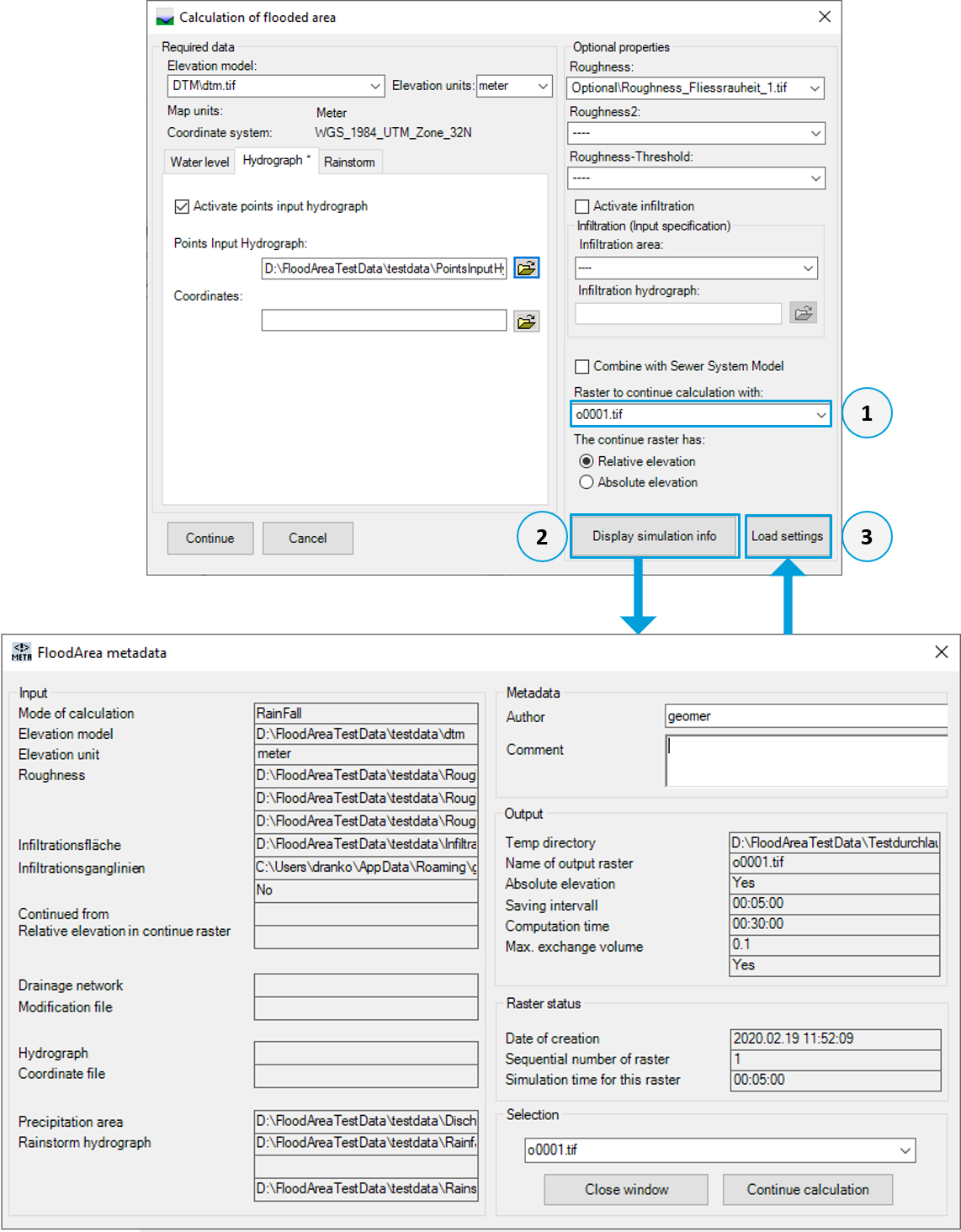
Continue calculation via the GUI is done via Display simulation info or directly by Calculate flooding areas . The button Load Settings in the main menu reads the settings from the metadata of the selected grid and writes them into the flood calculation dialog. Otherwise, the settings of the last calculation or already specified data are used. On the other hand, the settings of the dialog additional Settings are always automatically applied when a further calculation grid is specified, so that, for example, the same legend and the same saving interval are selected. If a change of the respective settings is desired, these must be made accordingly. The start time of the simulation is automatically set to the simulation time of the continuing calculation grid. The start time is interpreted as part of the specified simulation duration.
command line & toolbox
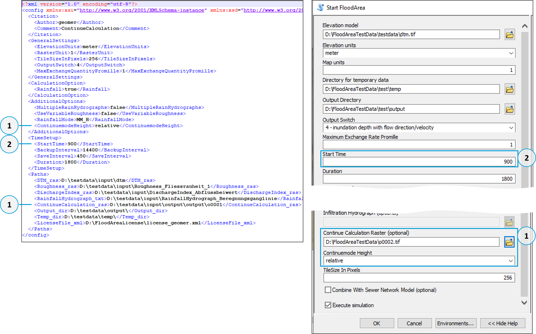
Both options are shown in the following figure (left via fng.xml, right via the toolbox). The grid for continue calculation is given as a path and it is indicated whether the flood depths are in relative elevation (water depth above ground level) or absolute elevation (including the DTM elevations plus water depth) (No. 2 in the screenshot). The start time must be adjusted as desired (No. 2, unit: seconds). Here the start time is interpreted as part of the specified simulation duration.
Combine with Sewer Network Model
cePipe - Sewer network modelling
cePipe is a software product from ce-tools - Civil Engineering Tools.
cePipe is a software product for the design and modeling of gravity sewers and pressure pipe networks. It is used in the fields of sewage disposal and water supply of the sanitary engineering. The software is easy to use and with a short training course it is quickly ready for use. cePipe is not a replacement for CAD programs or geographical information systems, but rather an extension for both systems. The program is to be seen as a supplement for the field of activity of a hydraulic engineer.
Further information can be found at https://ce-tools.at/index.php/produkte/cepipe. If you have questions about the software, you can reach Civil Engineering Tools at +43 (0) 664 23 23 522, Office@ce-tools.at.
Coupling with FloodArea HPC 11
The hydronumeric coupling of the 1D sewer network model cePipe with the 2D hydraulic simulation of FloodArea HPC 11 takes place via bidirectional coupling. Data is exchanged once every minute of the simulation time.
For the coupled simulation, cePipe and FloodArea HPC 11 must be installed on the same computer.
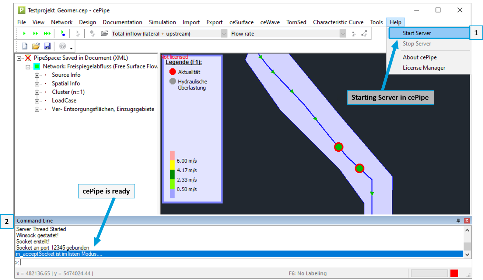
Please refer to the corresponding manual for data preparation for cePipe. The server must be started for the simulation:
1: under Help press Start Server
2: in the Command Line of cePipe you can now see if the server is ready. If it is, the line …is in listen mode… appears
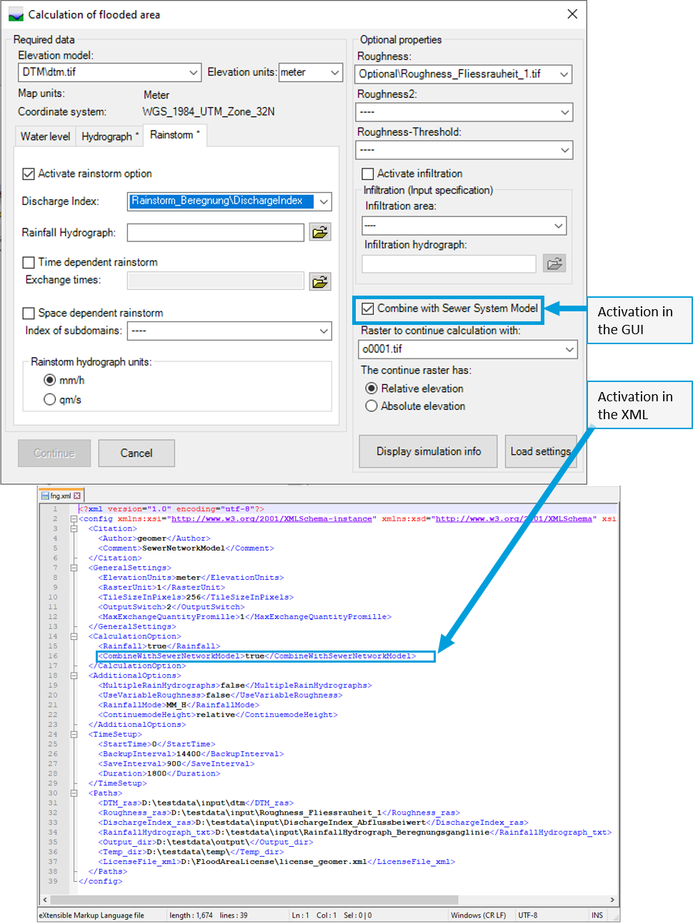
The simulation starts in both programs as soon as the FloodArea simulation is started. The following figure shows how the sewer network model is activated when FloodArea HPC 11 is started via the GUI and via the fng.xml. In the GUI, only the checkbox Enable coupling with sewer network model must be activated. In the fng.xml the line „<CombineWithSewerNetworkModel>true</CombineWithSewerNetworkModel>“ is inserted under CalculationOption according to the default by the Config.xsd.
If FloodArea is started via the toolbox, only the checkbox Combine With Sewer Network Model is activated. Then FloodArea HPC 11 can be started as usual.
